

Note
Go to the end to download the full example code.
Proximal solvers#
This example demonstrates the use of the solvers in the
pylops_mpi.proximal.optimization module.
import numpy as np
from mpi4py import MPI
from matplotlib import pyplot as plt

import pylops
import pyproximal

import pylops_mpi

plt.close("all")
comm = MPI.COMM_WORLD
rank = comm.Get_rank()
size = comm.Get_size()

np.random.seed(rank)
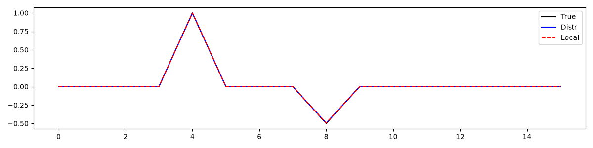
Let’s start with an example of sparsity promoting inversion using the
pylops_mpi.proximal.optimization.primal.ProximalGradient solver.
Here for illustrative purposes, we consider a case where the model is
broadcasted whilst the data is scattered across ranks.
# Sparse input
n = 16
arr = pylops_mpi.DistributedArray(
    global_shape=n,
    partition=pylops_mpi.Partition.BROADCAST)
arr[:] = 0.0
arr[n // 4] = 1.0
arr[n // 2] = -0.5

# Operator and data
A = np.random.normal(0, 1, (n // size, n,))
Opd = pylops_mpi.MPIVStack([pylops.MatrixMult(A), ])

b = Opd @ arr
blocal = b.asarray()

# L2 prox
l2d = pylops_mpi.proximal.MPIL2(
    Op=Opd, b=b, x0=arr.zeros_like())

# L1 prox
l1 = pyproximal.L1(sigma=1e-1)
l1d = pylops_mpi.proximal.MPIProxOperator(l1)

# Distributed inversion
arrpg = pylops_mpi.proximal.optimization.primal.ProximalGradient(
    l2d, l1d, x0=arr.zeros_like(), tau=1e-2, niter=400,
    show=True,
)
arrpgdlocal = arrpg.asarray()

# Benchmark serial inversion
As = np.vstack(comm.allgather(A))
arrlocal = arr.asarray()
if rank == 0:
    Op = pylops.MatrixMult(As)
    l2local = pyproximal.L2(
        Op=Op, b=blocal)
    l1local = pyproximal.L1(sigma=1e-1)

    arrpglocal = pyproximal.optimization.primal.ProximalGradient(
        l2local, l1local, x0=np.zeros(n), tau=1e-2, niter=400, show=False
    )

    plt.figure(figsize=(12, 3))
    plt.plot(arrlocal, "k", label="True")
    plt.plot(arrpgdlocal, "b", label="Distr")
    plt.plot(arrpglocal, "--r", label="Local")
    plt.legend()
    plt.tight_layout()
Accelerated Proximal Gradient
---------------------------------------------------------
Proximal operator (f): <MPIL2>
Proximal operator (g): <MPIProxOperator (L1)>
tau = 0.01      epsg = 1.0
niter = 400     tol = None
niterback = 100 acceleration = None

   Itn       x[0]          f           g       J=f+eps*g       tau
     1  -6.78097e-02   6.335e+00   1.141e-01   6.449e+00   1.000e-02
     2  -9.61259e-02   2.353e+00   1.728e-01   2.525e+00   1.000e-02
     3  -1.04538e-01   1.098e+00   2.055e-01   1.304e+00   1.000e-02
     4  -1.03219e-01   6.350e-01   2.234e-01   8.584e-01   1.000e-02
     5  -9.74574e-02   4.286e-01   2.333e-01   6.618e-01   1.000e-02
     6  -8.99726e-02   3.194e-01   2.386e-01   5.580e-01   1.000e-02
     7  -8.21326e-02   2.537e-01   2.413e-01   4.950e-01   1.000e-02
     8  -7.45942e-02   2.104e-01   2.424e-01   4.529e-01   1.000e-02
     9  -6.76431e-02   1.801e-01   2.426e-01   4.227e-01   1.000e-02
    10  -6.13744e-02   1.576e-01   2.421e-01   3.998e-01   1.000e-02
    41  -6.78370e-03   2.917e-02   2.051e-01   2.343e-01   1.000e-02
    81   0.00000e+00   9.089e-03   1.783e-01   1.874e-01   1.000e-02
   121   0.00000e+00   3.136e-03   1.590e-01   1.621e-01   1.000e-02
   161  -0.00000e+00   5.092e-04   1.495e-01   1.500e-01   1.000e-02
   201  -0.00000e+00   3.358e-04   1.493e-01   1.496e-01   1.000e-02
   241  -0.00000e+00   3.580e-04   1.493e-01   1.496e-01   1.000e-02
   281  -0.00000e+00   3.604e-04   1.493e-01   1.496e-01   1.000e-02
   321  -0.00000e+00   3.606e-04   1.493e-01   1.496e-01   1.000e-02
   361  -0.00000e+00   3.606e-04   1.493e-01   1.496e-01   1.000e-02
   392  -0.00000e+00   3.606e-04   1.493e-01   1.496e-01   1.000e-02
   393  -0.00000e+00   3.606e-04   1.493e-01   1.496e-01   1.000e-02
   394  -0.00000e+00   3.606e-04   1.493e-01   1.496e-01   1.000e-02
   395  -0.00000e+00   3.606e-04   1.493e-01   1.496e-01   1.000e-02
   396  -0.00000e+00   3.606e-04   1.493e-01   1.496e-01   1.000e-02
   397  -0.00000e+00   3.606e-04   1.493e-01   1.496e-01   1.000e-02
   398  -0.00000e+00   3.606e-04   1.493e-01   1.496e-01   1.000e-02
   399  -0.00000e+00   3.606e-04   1.493e-01   1.496e-01   1.000e-02
   400  -0.00000e+00   3.606e-04   1.493e-01   1.496e-01   1.000e-02

Total time (s) = 0.39
---------------------------------------------------------
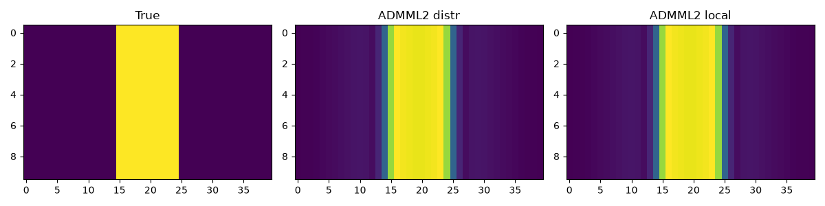
Next we use the pylops_mpi.proximal.optimization.primal.ADMML2
solver for a similar problem. However we consider here a 2d array and impose
blockiness in the solution. Once again, the model is broadcasted,
whilst the data is scattered.
# Input
ny, nx = 10 * size, 40
arrlocal = np.zeros((ny, nx))
arrlocal[ny // 2 - 5:ny // 2 + 5, nx // 2 - 5:nx // 2 + 5] = 2
arr = pylops_mpi.DistributedArray(
    global_shape=ny * nx,
    partition=pylops_mpi.Partition.BROADCAST
)
arr[:] = arrlocal.flatten()

# Operator and data
Op = pylops.VStack([pylops.Diagonal(np.ones(ny * nx)) for _ in range(size)])
Opd = pylops_mpi.MPIVStack([pylops.Diagonal(np.ones(ny * nx)),])

b = Opd @ arr
blocal = b.asarray()

# Regularizer
Gopd = pylops_mpi.MPILinearOperator(pylops.Gradient(
    dims=(ny, nx), sampling=1., edge=False, kind="forward"))

l1 = pyproximal.L1(sigma=2e0)
l1d = pylops_mpi.proximal.MPIProxOperator(l1)

# Distributed inversion
L = 8.0  # max eig of Gopd.H @ Gop
x0distr = arr.zeros_like()
arradmm = pylops_mpi.proximal.optimization.primal.ADMML2(
    l1d, Opd, b, Gopd, x0=x0distr, tau=.99 / L, niter=5,
    show=True, kwargs_solver=dict(niter=5),
)[0]
arradmmdlocal = arradmm.asarray()

# Benchmark serial inversion
arrlocal = arr.asarray()
if rank == 0:

    Gop = pylops.Gradient(
        dims=(ny, nx), sampling=1., edge=False, kind="forward",
    )
    l1local = pyproximal.L1(sigma=2e0)

    arradmmlocal = pyproximal.optimization.primal.ADMML2(
        l1local, Op, blocal, Gop, x0=np.zeros(ny * nx),
        tau=.99 / L, niter=5, show=False, iter_lim=5,
    )[0]

    fig, axs = plt.subplots(1, 3, figsize=(12, 3))
    axs[0].imshow(arrlocal.reshape(10 * size, 40))
    axs[0].set_title("True")
    axs[0].axis("tight")
    axs[1].imshow(arradmmdlocal.reshape(10 * size, 40))
    axs[1].set_title("ADMML2 distr")
    axs[1].axis("tight")
    axs[2].imshow(arradmmlocal.reshape(10 * size, 40))
    axs[2].set_title("ADMML2 local")
    axs[2].axis("tight")
    fig.tight_layout()
ADMM
---------------------------------------------------------
Proximal operator (g): <MPIProxOperator (L1)>
tau = 1.237500e-01      niter = 5

   Itn       x[0]          f           g       J = f + g
     1   0.00000e+00   2.658e+01   6.862e+01   9.520e+01
     2   0.00000e+00   4.653e+01   5.350e+01   1.000e+02
     3   0.00000e+00   3.575e+01   5.484e+01   9.058e+01
     4   6.54288e-02   2.735e+01   5.783e+01   8.518e+01
     5   1.08365e-01   2.254e+01   6.021e+01   8.274e+01

Total time (s) = 0.07
---------------------------------------------------------
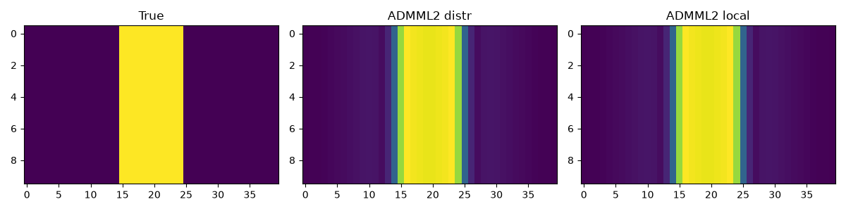
And finally we repeat the same with a scattered model.
# Input
ny, nx = 10 * size, 40
arrlocal = np.zeros((ny, nx))
arrlocal[ny // 2 - 5:ny // 2 + 5, nx // 2 - 5:nx // 2 + 5] = 2
arr = pylops_mpi.DistributedArray(global_shape=ny * nx,
                                  partition=pylops_mpi.Partition.SCATTER)
arr[:] = arrlocal[ny // size * rank: ny // size * (rank + 1)].flatten()

# Operator and data
Op = pylops.Diagonal(np.ones(ny * nx))
Opd = pylops_mpi.MPIBlockDiag([pylops.Diagonal(np.ones((ny * nx) // size)),])

b = Opd @ arr
blocal = b.asarray()

# Regularizer
Gopd = pylops_mpi.MPIGradient(
    dims=(ny, nx), sampling=1., edge=False, kind="forward")

l1 = pyproximal.L1(sigma=2e0)
l1d = pylops_mpi.proximal.MPIProxOperator(l1)

# Distributed inversion
L = 8.0  # max eig of Gopd.H @ Gop
x0distr = arr.zeros_like()
arradmm = pylops_mpi.proximal.optimization.primal.ADMML2(
    l1d, Opd, b, Gopd, x0=x0distr, tau=.99 / L, niter=5,
    show=True, kwargs_solver=dict(niter=5),
)[0]
arradmmdlocal = arradmm.asarray()

# Benchmark serial inversion
arrlocal = arr.asarray()
if rank == 0:

    Gop = pylops.Gradient(
        dims=(ny, nx), sampling=1., edge=False, kind="forward"
    )
    l1local = pyproximal.L1(sigma=2e0)

    arradmmlocal = pyproximal.optimization.primal.ADMML2(
        l1local, Op, blocal, Gop, x0=np.zeros(ny * nx),
        tau=.99 / L, niter=5, show=False, iter_lim=5,
    )[0]

    fig, axs = plt.subplots(1, 3, figsize=(12, 3))
    axs[0].imshow(arrlocal.reshape(10 * size, 40))
    axs[0].set_title("True")
    axs[0].axis("tight")
    axs[1].imshow(arradmmdlocal.reshape(10 * size, 40))
    axs[1].set_title("ADMML2 distr")
    axs[1].axis("tight")
    axs[2].imshow(arradmmlocal.reshape(10 * size, 40))
    axs[2].set_title("ADMML2 local")
    axs[2].axis("tight")
    fig.tight_layout()
ADMM
---------------------------------------------------------
Proximal operator (g): <MPIProxOperator (L1)>
tau = 1.237500e-01      niter = 5

   Itn       x[0]          f           g       J = f + g
     1   0.00000e+00   2.658e+01   6.862e+01   9.520e+01
     2   0.00000e+00   4.653e+01   5.350e+01   1.000e+02
     3   0.00000e+00   3.575e+01   5.484e+01   9.058e+01
     4   6.54288e-02   2.735e+01   5.783e+01   8.518e+01
     5   1.08365e-01   2.254e+01   6.021e+01   8.274e+01

Total time (s) = 0.18
---------------------------------------------------------
Total running time of the script: (0 minutes 1.172 seconds)