Derivatives

This example demonstrates how to use pylops-mpi’s derivative operators, namely pylops_mpi.basicoperators.MPIFirstDerivative, pylops_mpi.basicoperators.MPISecondDerivative and pylops_mpi.basicoperators.MPILaplacian.

We will be focusing here on the case where the input array \(x\) is assumed to be an n-dimensional pylops_mpi.DistributedArray and the derivative is applied over the first axis (axis=0). Since the array is distributed over multiple processes, the derivative operators must take care of applying the derivatives across the edges using the information from the previous/next processes, using the so-called ghost cells.

Derivative operators are commonly used when solving inverse problems within regularization terms aimed at enforcing smooth solutions

from matplotlib import pyplot as plt
import numpy as np
from mpi4py import MPI

import pylops_mpi

plt.close("all")
np.random.seed(42)

rank = MPI.COMM_WORLD.Get_rank()
size = MPI.COMM_WORLD.Get_size()

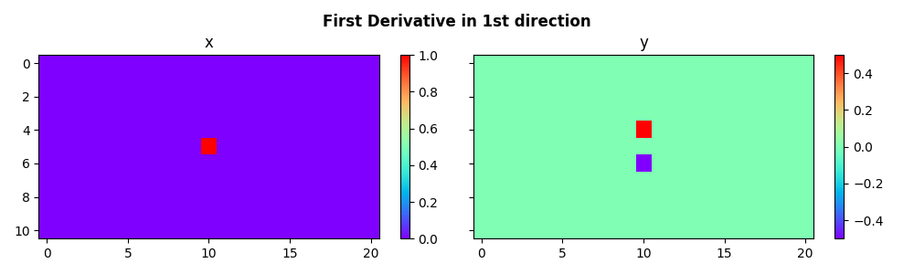
Let’s start by applying the first derivative on a pylops_mpi.DistributedArray in the first direction(i.e. along axis=0) using the pylops_mpi.basicoperators.MPIFirstDerivative operator.

nx, ny = 11, 21
x = np.zeros((nx, ny))
x[nx // 2, ny // 2] = 1.0

Fop = pylops_mpi.MPIFirstDerivative((nx, ny), dtype=np.float64)
x_dist = pylops_mpi.DistributedArray.to_dist(x=x.flatten())
y_dist = Fop @ x_dist
y = y_dist.asarray().reshape((nx, ny))

if rank == 0:
    fig, axs = plt.subplots(1, 2, figsize=(10, 3), sharey=True)
    fig.suptitle(
        "First Derivative in 1st direction", fontsize=12, fontweight="bold", y=0.95
    )
    im = axs[0].imshow(x, interpolation="nearest", cmap="rainbow")
    axs[0].axis("tight")
    axs[0].set_title("x")
    plt.colorbar(im, ax=axs[0])
    im = axs[1].imshow(y, interpolation="nearest", cmap="rainbow")
    axs[1].axis("tight")
    axs[1].set_title("y")
    plt.colorbar(im, ax=axs[1])
    plt.tight_layout()
    plt.subplots_adjust(top=0.8)

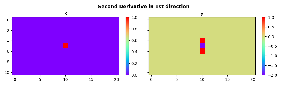
We can now do the same for the second derivative using the pylops_mpi.basicoperators.MPISecondDerivative operator.

nx, ny = 11, 21
x = np.zeros((nx, ny))
x[nx // 2, ny // 2] = 1.0

Sop = pylops_mpi.MPISecondDerivative(dims=(nx, ny), dtype=np.float64)
x_dist = pylops_mpi.DistributedArray.to_dist(x=x.flatten())
y_dist = Sop @ x_dist
y = y_dist.asarray().reshape((nx, ny))

if rank == 0:
    fig, axs = plt.subplots(1, 2, figsize=(10, 3), sharey=True)
    fig.suptitle(
        "Second Derivative in 1st direction", fontsize=12, fontweight="bold", y=0.95
    )
    im = axs[0].imshow(x, interpolation="nearest", cmap="rainbow")
    axs[0].axis("tight")
    axs[0].set_title("x")
    plt.colorbar(im, ax=axs[0])
    im = axs[1].imshow(y, interpolation="nearest", cmap="rainbow")
    axs[1].axis("tight")
    axs[1].set_title("y")
    plt.colorbar(im, ax=axs[1])
    plt.tight_layout()
    plt.subplots_adjust(top=0.8)

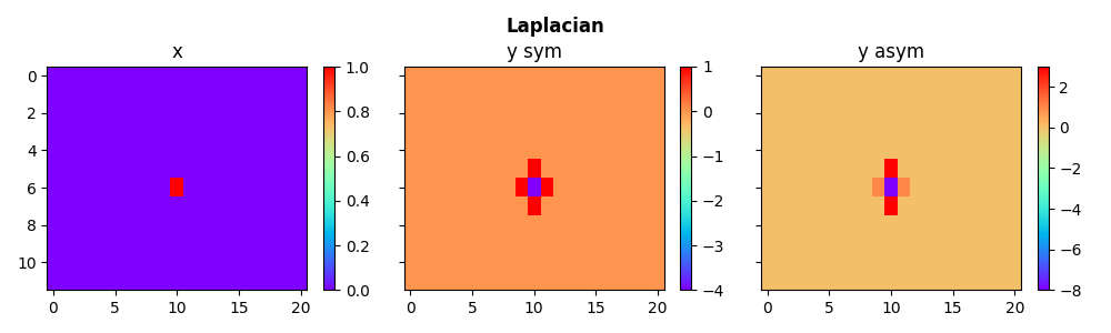
We now use the pylops_mpi.basicoperators.MPILaplacian to calculate second derivative along two directions of the distributed array. We use a symmetrical as well as an asymmetrical (adding more weight to the derivative along one direction) version to achieve this.

nx, ny = (12, 21)
x = np.zeros((nx, ny))
x[nx // 2, ny // 2] = 1.0

# Symmetrical
L2symop = pylops_mpi.MPILaplacian(dims=(nx, ny), weights=(1, 1), dtype=np.float64)

# Asymmetrical
L2asymop = pylops_mpi.MPILaplacian(dims=(nx, ny), weights=(3, 1), dtype=np.float64)

x_dist = pylops_mpi.DistributedArray.to_dist(x=x.flatten())
ysym_dist = L2symop @ x_dist
ysym = ysym_dist.asarray().reshape((nx, ny))
yasym_dist = L2asymop @ x_dist
yasym = yasym_dist.asarray().reshape((nx, ny))

if rank == 0:
    fig, axs = plt.subplots(1, 3, figsize=(10, 3), sharey=True)
    fig.suptitle("Laplacian", fontsize=12, fontweight="bold", y=0.95)
    im = axs[0].imshow(x, interpolation="nearest", cmap="rainbow")
    axs[0].axis("tight")
    axs[0].set_title("x")
    plt.colorbar(im, ax=axs[0])
    im = axs[1].imshow(ysym, interpolation="nearest", cmap="rainbow")
    axs[1].axis("tight")
    axs[1].set_title("y sym")
    plt.colorbar(im, ax=axs[1])
    im = axs[2].imshow(yasym, interpolation="nearest", cmap="rainbow")
    axs[2].axis("tight")
    axs[2].set_title("y asym")
    plt.colorbar(im, ax=axs[2])
    plt.tight_layout()
    plt.subplots_adjust(top=0.8)

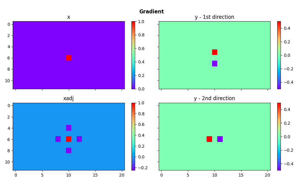
We now consider the pylops_mpi.basicoperators.MPIGradient operator. Given a 2-dimensional array, this operator applies first-order derivatives on both dimensions and concatenates them.

Gop = pylops_mpi.MPIGradient(dims=(nx, ny), dtype=np.float64)

y_grad_dist = Gop @ x_dist
# Reshaping to (ndims, nx, ny) for plotting
y_grad = y_grad_dist.asarray().reshape((2, nx, ny))
y_grad_adj_dist = Gop.H @ y_grad_dist
# Reshaping to (nx, ny) for plotting
y_grad_adj = y_grad_adj_dist.asarray().reshape((nx, ny))

if rank == 0:
    fig, axs = plt.subplots(2, 2, figsize=(10, 6), sharex=True, sharey=True)
    fig.suptitle("Gradient", fontsize=12, fontweight="bold", y=0.95)
    im = axs[0, 0].imshow(x, interpolation="nearest", cmap="rainbow")
    axs[0, 0].axis("tight")
    axs[0, 0].set_title("x")
    plt.colorbar(im, ax=axs[0, 0])
    im = axs[0, 1].imshow(y_grad[0, ...], interpolation="nearest", cmap="rainbow")
    axs[0, 1].axis("tight")
    axs[0, 1].set_title("y - 1st direction")
    plt.colorbar(im, ax=axs[0, 1])
    im = axs[1, 1].imshow(y_grad[1, ...], interpolation="nearest", cmap="rainbow")
    axs[1, 1].axis("tight")
    axs[1, 1].set_title("y - 2nd direction")
    plt.colorbar(im, ax=axs[1, 1])
    im = axs[1, 0].imshow(y_grad_adj, interpolation="nearest", cmap="rainbow")
    axs[1, 0].axis("tight")
    axs[1, 0].set_title("xadj")
    plt.colorbar(im, ax=axs[1, 0])
    plt.tight_layout()