Fourier Transform

This example shows how to use the pylops_mpi.signalprocessing.MPIFFT2D and pylops_mpi.signalprocessing.MPIFFTND operators to apply the Fourier Transform to the model and the inverse Fourier Transform to the data.

import matplotlib.pyplot as plt
import numpy as np

import pylops_mpi

plt.close("all")

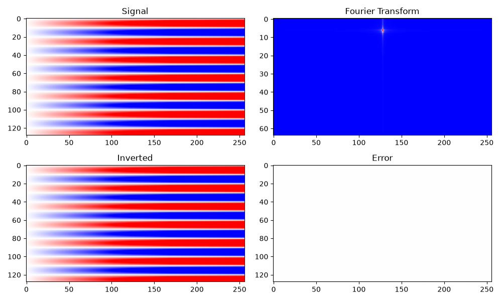
We start by applying the two dimensional MPI-distributed FFT to a two-dimensional signal using pylops_mpi.signalprocessing.MPIFFT2D. The input signal is a pylops_mpi.DistributedArray which is distributed across MPI ranks before applying the transform.

dt, dx = 0.005, 5
nt, nx = 2**7, 2**8
t = np.arange(nt) * dt
x = np.arange(nx) * dx
f0 = 10

d = np.outer(np.sin(2 * np.pi * f0 * t), np.arange(nx) + 1)
dist = pylops_mpi.DistributedArray.to_dist(x=d.ravel())

FFTop = pylops_mpi.signalprocessing.MPIFFT2D(
    dims=(nt, nx), sampling=(dt, dx)
)

D = FFTop * dist

dinv = FFTop / D
dinv = np.real(dinv.asarray()).reshape(nt, nx)

D_2d = D.asarray().reshape(nt, nx)

fig, axs = plt.subplots(2, 2, figsize=(10, 6))

axs[0][0].imshow(d, vmin=-100, vmax=100, cmap="bwr")
axs[0][0].set_title("Signal")
axs[0][0].axis("tight")

axs[0][1].imshow(
    np.abs(np.fft.fftshift(D_2d, axes=1)[:nt // 2, :]), cmap="bwr"
)
axs[0][1].set_title("Fourier Transform")
axs[0][1].axis("tight")

axs[1][0].imshow(dinv, vmin=-100, vmax=100, cmap="bwr")
axs[1][0].set_title("Inverted")
axs[1][0].axis("tight")

axs[1][1].imshow(d - dinv, vmin=-100, vmax=100, cmap="bwr")
axs[1][1].set_title("Error")
axs[1][1].axis("tight")

fig.tight_layout()

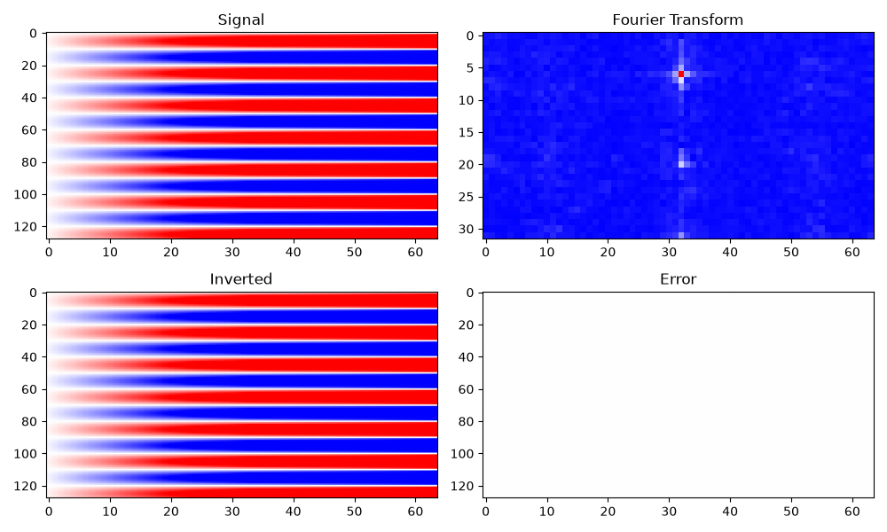
We can also apply the three dimensional MPI-distributed FFT to a three-dimensional signal using pylops_mpi.signalprocessing.MPIFFTND.

dt, dx, dy = 0.005, 5, 3
nt, nx, ny = 2**7, 2**6, 13
t = np.arange(nt) * dt
x = np.arange(nx) * dx
y = np.arange(ny) * dy
f0 = 10

d = np.outer(np.sin(2 * np.pi * f0 * t), np.arange(nx) + 1)
d = np.tile(d[:, :, np.newaxis], [1, 1, ny])
dist = pylops_mpi.DistributedArray.to_dist(x=d.ravel())

FFTop = pylops_mpi.signalprocessing.MPIFFTND(
    dims=(nt, nx, ny),
    sampling=(dt, dx, dy)
)

D = FFTop * dist
dinv = FFTop / D
dinv = np.real(dinv.asarray()).reshape(nt, nx, ny)
D_3d = D.asarray().reshape(nt, nx, ny)  # shape matches dims now

fig, axs = plt.subplots(2, 2, figsize=(10, 6))

axs[0][0].imshow(d[:, :, ny // 2], vmin=-20, vmax=20, cmap="bwr")
axs[0][0].set_title("Signal")
axs[0][0].axis("tight")
axs[0][1].imshow(
    np.abs(np.fft.fftshift(D_3d, axes=1)[:nx // 2, :, ny // 2]),
    cmap="bwr"
)
axs[0][1].set_title("Fourier Transform")
axs[0][1].axis("tight")

axs[1][0].imshow(dinv[:, :, ny // 2], vmin=-20, vmax=20, cmap="bwr")
axs[1][0].set_title("Inverted")
axs[1][0].axis("tight")

axs[1][1].imshow(d[:, :, ny // 2] - dinv[:, :, ny // 2], vmin=-20, vmax=20, cmap="bwr")
axs[1][1].set_title("Error")
axs[1][1].axis("tight")

fig.tight_layout()