MPILinearOperator

This example demonstrates the use of the pylops_mpi.MPILinearOperator to wrap PyLops Operators. PyLops operators can be converted into pylops_mpi.MPILinearOperator using the pylops_mpi.asmpilinearoperator method. Additionally, the example showcases how to use these wrapped PyLops operators with other operators provided by PyLops-MPI.

import numpy as np
from mpi4py import MPI
from matplotlib import pyplot as plt

import pylops

import pylops_mpi

np.random.seed(42)
plt.close("all")
rank = MPI.COMM_WORLD.Get_rank()
size = MPI.COMM_WORLD.Get_size()

Let’s start by creating an instance of the pylops.FirstDerivative, which we will then convert into an MPILinearOperator using the pylops_mpi.asmpilinearoperator method.

Ny, Nx = 11, 22
Fop = pylops.FirstDerivative(dims=(Ny, Nx), axis=0, dtype=np.float64)
Mop = pylops_mpi.asmpilinearoperator(Op=Fop)
print(Mop)

<242x242 MPILinearOperator with dtype=float64>

Now, to carry out the matrix-vector product using the MPILinearOperator, we first create a pylops_mpi.DistributedArray with the partition set to pylops_mpi.Partition.BROADCAST, denoted by \(x\). The matrix-vector product is then computed at each rank, and the result returned is a pylops_mpi.DistributedArray with the same partitioning.

x = pylops_mpi.DistributedArray(global_shape=Ny * Nx, partition=pylops_mpi.Partition.BROADCAST)
x[:] = 1
y = Mop @ x
print(f'y: {y}')

y: <DistributedArray with global shape=(242,), local shape=(242,), dtype=float64, processes=[0])>

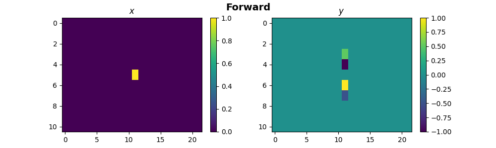
Next, we can take the MPILinearOperator and combine it with other operators provided by pylops_mpi to create more advanced MPI operators. In this example, we’ll combine the pylops_mpi.MPILinearOperator with the pylops_mpi.basicoperators.MPIVStack and perform matrix-vector multiplication and adjoint matrix-vector multiplication.

Sop = pylops.SecondDerivative(dims=(Ny, Nx), axis=0, dtype=np.float64)
VStack = pylops_mpi.MPIVStack(ops=[(rank + 1) * Sop, ])
FullOp = VStack @ Mop

To perform the matrix vector multiplication on the full operator, we will use a pylops_mpi.DistributedArray with partition set to pylops_mpi.Partition.BROADCAST.

X = np.zeros(shape=(Ny, Nx))
X[Ny // 2, Nx // 2] = 1
X1 = X.ravel()
x = pylops_mpi.DistributedArray(global_shape=Ny * Nx, partition=pylops_mpi.Partition.BROADCAST)
x[:] = X1
y_dist = FullOp @ x
y = y_dist.asarray().reshape((size * Ny, Nx))
if rank == 0:
    fig, ax = plt.subplots(nrows=1, ncols=2, figsize=(10, 3))
    im1 = ax[0].imshow(X, interpolation="nearest")
    ax[0].set_title("$x$")
    ax[0].axis("tight")
    fig.colorbar(im1, ax=ax[0])
    im2 = ax[1].imshow(y, interpolation="nearest")
    ax[1].set_title("$y$")
    ax[1].axis("tight")
    fig.colorbar(im2, ax=ax[1])
    fig.suptitle("Forward", fontsize=14, fontweight="bold")

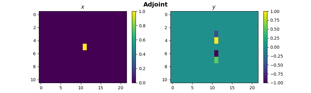
For adjoint matrix-vector multiplication, we will use a pylops_mpi.DistributedArray with the partition set to pylops_mpi.Partition.SCATTER. It is essential to ensure that the operators align appropriately with their corresponding \(x\) during this process.

x = pylops_mpi.DistributedArray(global_shape=size * Ny * Nx, partition=pylops_mpi.Partition.SCATTER)
x[:] = X1
y_dist = FullOp.H @ x
y = y_dist.asarray().reshape((Ny, Nx))
if rank == 0:
    fig, ax = plt.subplots(nrows=1, ncols=2, figsize=(10, 3))
    im1 = ax[0].imshow(X, interpolation="nearest")
    ax[0].set_title("$x$")
    ax[0].axis("tight")
    fig.colorbar(im1, ax=ax[0])
    im2 = ax[1].imshow(y, interpolation="nearest")
    ax[1].set_title("$y$")
    ax[1].axis("tight")
    fig.colorbar(im2, ax=ax[1])
    fig.suptitle("Adjoint", fontsize=14, fontweight="bold")