Stacking Operators

This example shows how to use “stacking” operators such as pylops_mpi.basicoperators.MPIVStack, pylops_mpi.basicoperators.MPIHStack and pylops_mpi.basicoperators.MPIBlockDiag.

The operators mentioned above enable the input of various linear operators within a single operator. PyLops-MPI utilizes these operators to construct complex operators that are used in various optimization problems involving regularization and preconditioning.

Within PyLops-MPI, the pylops_mpi.DistributedArray is utilized to compute the matrix-vector product for each operator contained within the stacking operators. At each rank, every individual operator, or a list of operators, performs its matrix-vector product in a distributed manner. Subsequently, the operation returns a pylops_mpi.DistributedArray. To obtain the global NumPy array from the DistributedArray, you can use the asarray() method.

import numpy as np
from mpi4py import MPI
from matplotlib import pyplot as plt

import pylops

import pylops_mpi

np.random.seed(42)
plt.close("all")
rank = MPI.COMM_WORLD.Get_rank()
size = MPI.COMM_WORLD.Get_size()

Let’s start by defining two instances of the pylops.SecondDerivative which will be used in this example.

D2hop = pylops.SecondDerivative(dims=(11, 22), axis=1, dtype=np.float64)
D2vop = pylops.SecondDerivative(dims=(11, 22), axis=0, dtype=np.float64)

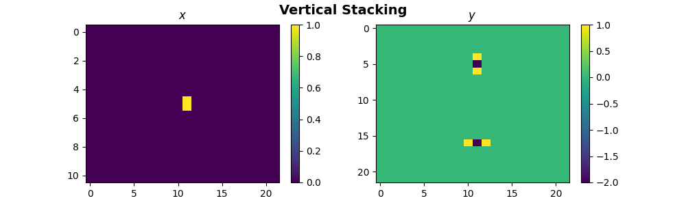
Now, we will look at vertical stacking using the pylops_mpi.basicoperators.MPIVStack operator.

\[\begin{split}\mathbf{D_{Vstack}} = \begin{bmatrix} \mathbf{D_{v}} \\ \mathbf{D_{h}} \\ \vdots \\ (i+1) * \mathbf{D_{v}} \\ (i+1) * \mathbf{D_{h}} \\ \end{bmatrix}, \qquad \mathbf{y} = \begin{bmatrix} \mathbf{D_{v}}\mathbf{x} \\ \mathbf{D_{h}}\mathbf{x} \\ \vdots \\ (i+1) * \mathbf{D_{v}}\mathbf{x} \\ (i+1) * \mathbf{D_{h}}\mathbf{x} \\ \end{bmatrix}\end{split}\]

At each rank, the MPIVStack operator takes two operators, \((i+1) * \mathbf{D_{v}}\) and \((i+1) * \mathbf{D_{h}}\), where each rank is indicated by \(i\). In this example, the model vector, \(x\), is represented as a pylops_mpi.DistributedArray with the partition set to pylops_mpi.Partition.BROADCAST. At each rank, a matrix-vector product is performed in the forward mode, and the result is stored in the variable \(y\).

Nv, Nh = (11, 22)
X = np.zeros(shape=(Nv, Nh))
X[Nv // 2, Nh // 2] = 1
X1 = X.ravel()
x = pylops_mpi.DistributedArray(global_shape=Nv * Nh, partition=pylops_mpi.Partition.BROADCAST)
x[:] = X1
VStack = pylops_mpi.MPIVStack(ops=[(rank + 1) * D2vop, (rank + 1) * D2hop])
y = VStack @ x
y_array = y.asarray().reshape(2 * size * Nv, Nh)

if rank == 0:
    # Visualize
    fig, ax = plt.subplots(nrows=1, ncols=2, figsize=(10, 3))
    im1 = ax[0].imshow(X, interpolation="nearest")
    ax[0].set_title("$x$")
    ax[0].axis("tight")
    fig.colorbar(im1, ax=ax[0])
    im2 = ax[1].imshow(y_array, interpolation="nearest")
    ax[1].set_title("$y$")
    ax[1].axis("tight")
    fig.colorbar(im2, ax=ax[1])
    fig.suptitle("Vertical Stacking", fontsize=14, fontweight="bold")

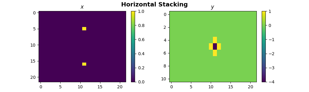
Now, let’s take a look at the pylops_mpi.basicoperators.MPIHStack operator, which is specifically designed to horizontally stack linear operators in a distributed fashion.

\[\begin{split}\mathbf{D_{Hstack}} = \begin{bmatrix} \mathbf{D_{v}} & \mathbf{D_{h}} & \ldots & (i+1) * \mathbf{D_{v}} & (i+1) * \mathbf{D_{h}} \\ \end{bmatrix} \qquad \\ \\ \mathbf{y} = \begin{bmatrix} \mathbf{D_{v}}\mathbf{x_{1}} + \mathbf{D_{h}}\mathbf{x_{2}} + \ldots + (i+1) * \mathbf{D_{v}}\mathbf{x_{n-1}} + (i+1) * \mathbf{D_{h}}\mathbf{x_{n}} \\ \end{bmatrix}\end{split}\]

Similar to the MPIVStack, the MPIHStack also contains two operators at each rank, and the model vector \(x\) is a DistributedArray, but this time the partition is set to pylops_mpi.Partition.SCATTER. Each operator performs the matrix-vector product with its corresponding \(x\). The final result undergoes a sum-reduction, and is stored in the variable \(y\).

Nv, Nh = (11, 22)
X = np.zeros(shape=(Nv * 2, Nh))
X[Nv // 2, Nh // 2] = 1
X[Nv // 2 + Nv, Nh // 2] = 1
X1 = X.ravel()
x = pylops_mpi.DistributedArray(global_shape=2 * size * Nv * Nh, partition=pylops_mpi.Partition.SCATTER)
x[:] = X1
HStack = pylops_mpi.MPIHStack(ops=[(rank + 1) * D2vop, (rank + 1) * D2hop])
y = HStack @ x
y_array = y.asarray().reshape(Nv, Nh)

if rank == 0:
    # Visualize
    fig, ax = plt.subplots(nrows=1, ncols=2, figsize=(10, 3))
    im1 = ax[0].imshow(X, interpolation="nearest")
    ax[0].set_title("$x$")
    ax[0].axis("tight")
    fig.colorbar(im1, ax=ax[0])
    im2 = ax[1].imshow(y_array, interpolation="nearest")
    ax[1].set_title("$y$")
    ax[1].axis("tight")
    fig.colorbar(im2, ax=ax[1])
    fig.suptitle("Horizontal Stacking", fontsize=14, fontweight="bold")

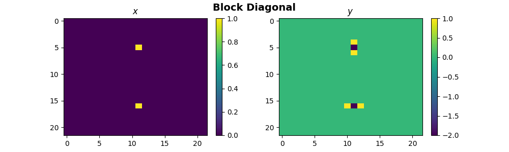
Finally, we can use the pylops_mpi.basicoperators.MPIBlockDiag to apply operators to different subset of the model and data.

\[\begin{split}\mathbf{D_{BDiag}} = \begin{bmatrix} \mathbf{D_{v}} & \mathbf{0} & \ldots &\ldots & \mathbf{0} \\ \mathbf{0} & \mathbf{D_{h}} & \ldots & \ldots & \mathbf{0} \\ \vdots & \vdots & \ddots & \ldots & \vdots \\ \vdots & \vdots & \ldots & (i+1) * \mathbf{D_{v}} & \vdots \\ \mathbf{0} & \mathbf{0} & \ldots & \ldots & (i+1) * \mathbf{D_{h}} \\ \end{bmatrix} \qquad \mathbf{y} = \begin{bmatrix} \mathbf{D_{v}}\mathbf{x_{1}} \\ \mathbf{D_{h}}\mathbf{x_{2}} \\ \vdots \\ (i+1) * \mathbf{D_{v}}\mathbf{x_{n-1}} \\ (i+1) * \mathbf{D_{h}}\mathbf{x_{n}} \\ \end{bmatrix}\end{split}\]

Each operator performs its matrix-vector product in forward mode with its corresponding vector \(x\).

Nv, Nh = (11, 22)
BDiag = pylops_mpi.MPIBlockDiag(ops=[(rank + 1) * D2vop, (rank + 1) * D2hop])
y = BDiag @ x
y_array = y.asarray().reshape(2 * size * Nv, Nh)

if rank == 0:
    # Visualize
    fig, ax = plt.subplots(nrows=1, ncols=2, figsize=(10, 3))
    im1 = ax[0].imshow(X, interpolation="nearest")
    ax[0].set_title("$x$")
    ax[0].axis("tight")
    fig.colorbar(im1, ax=ax[0])
    im2 = ax[1].imshow(y_array, interpolation="nearest")
    ax[1].set_title("$y$")
    ax[1].axis("tight")
    fig.colorbar(im2, ax=ax[1])
    fig.suptitle("Block Diagonal", fontsize=14, fontweight="bold")