Non-Stationary Convolution

This example demonstrates how to use the pylops_mpi.signalprocessing.MPINonStationaryConvolve1D operator to apply 1d non-stationary convolution to 1-dimensional or N-dimensional distributed arrays over the distributed axis.

This operator is effectively equivalent to PyLops’ pylops.signalprocessing.NonStationaryConvolve1D, however both the input array and the filters will be distibuted. What makes this operator interesting is that we need to handle convolutions at the edges between different ranks and to do that we will halo the input array of a number of samples equal to the distance between two filters and we will also borrow the filtering from the next/previous rank. This is internally achieved by means of the pylops_mpi.basicoperators.MPIHalo operator.

from matplotlib import pyplot as plt

import sys
import time
import numpy as np
import pylops

from pylops.utils.wavelets import ricker
from mpi4py import MPI

import pylops_mpi

plt.close("all")
np.random.seed(42)

comm = MPI.COMM_WORLD
rank = comm.Get_rank()
size = comm.Get_size()

def pause(comm, t=4):
    sys.stdout.flush()
    comm.barrier()
    time.sleep(t)

def local_extent_from_slice(local_shape, local_slice, halo):
    lefts = []
    rights = []
    if isinstance(halo, int):
        for sl in local_slice:
            lefts.append(halo if (sl.start or 0) > 0 else 0)
            rights.append(halo if sl.stop is not None else 0)
    else:
        for sl, hal in zip(local_slice, halo):
            lefts.append(hal if (sl.start or 0) > 0 else 0)
            rights.append(hal if sl.stop is not None else 0)
    extent = tuple(dim + l + r for dim, l, r in zip(local_shape, lefts, rights))
    return extent, lefts, rights

Let’s start by creating a 1-dimensional distruted array as well as the filters

# Input signal dimensions
nlocal = 64
nfilters_local = 4
n = nlocal * size
proc_grid_shape = (size, )

# Filters
ntw = 16
dt = 0.004
tw = np.arange(ntw) * dt
fs = np.arange(nfilters_local * size) * 8 + 20
wavs = np.stack([ricker(tw, f0=f)[0] for f in fs])

# Filters centers (selected such that they are symmetric on either
# side of the edges of the distributed array between ranks)
n_between_h = nlocal // nfilters_local
ih = nlocal // (2 * nfilters_local) + \
    np.arange(0, nlocal * size, n_between_h)

pause(comm, t=1)
if rank == 0:
    print(f"Filters centers: {ih}")

# Input signal
t = np.arange(n) * dt
x = np.zeros(n, dtype=np.float64)
x[ih] = 1.0

# Distributed array
x_dist = pylops_mpi.DistributedArray(
    global_shape=n,
    base_comm=comm,
    partition=pylops_mpi.Partition.SCATTER)
x_dist.local_array[:] = x[nlocal * rank: nlocal * (rank + 1)]

# Create operator
COp_dist = pylops_mpi.signalprocessing.MPINonStationaryConvolve1D(
    n, wavs, ih, base_comm=comm)

# Apply operator
y_dist = COp_dist @ x_dist
xadj_dist = COp_dist.H @ y_dist

y_dist = y_dist.asarray()
xadj_dist = xadj_dist.asarray()

# Create and apply benchmark serial operator
COp = pylops.signalprocessing.NonStationaryConvolve1D(
    dims=n, hs=wavs, ih=ih
)

y = COp @ x
xadj = COp.H @ y

/opt/hostedtoolcache/Python/3.11.15/x64/lib/python3.11/site-packages/pylops/utils/wavelets.py:196: UserWarning: One sample removed from time axis...
  t = _tcrop(t)
Filters centers: [ 8 24 40 56]

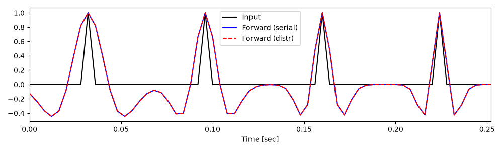
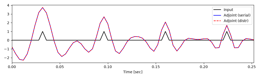
Let’s display the results

if rank == 0:
    plt.figure(figsize=(10, 3))
    plt.plot(t, x, "k", label="Input")
    plt.plot(t, y, "b", label="Forward (serial)")
    plt.plot(t, y_dist, "--r", label="Forward (distr)")
    plt.xlabel("Time [sec]")
    plt.xlim(0, t[-1])
    plt.legend()
    plt.tight_layout()

    plt.figure(figsize=(10, 3))
    plt.plot(t, x, "k", label="Input")
    plt.plot(t, xadj, "b", label="Adjoint (serial)")
    plt.plot(t, xadj_dist, "--r", label="Adjoint (distr)")
    plt.xlabel("Time [sec]")
    plt.xlim(0, t[-1])
    plt.legend()
    plt.tight_layout()

• 
• 

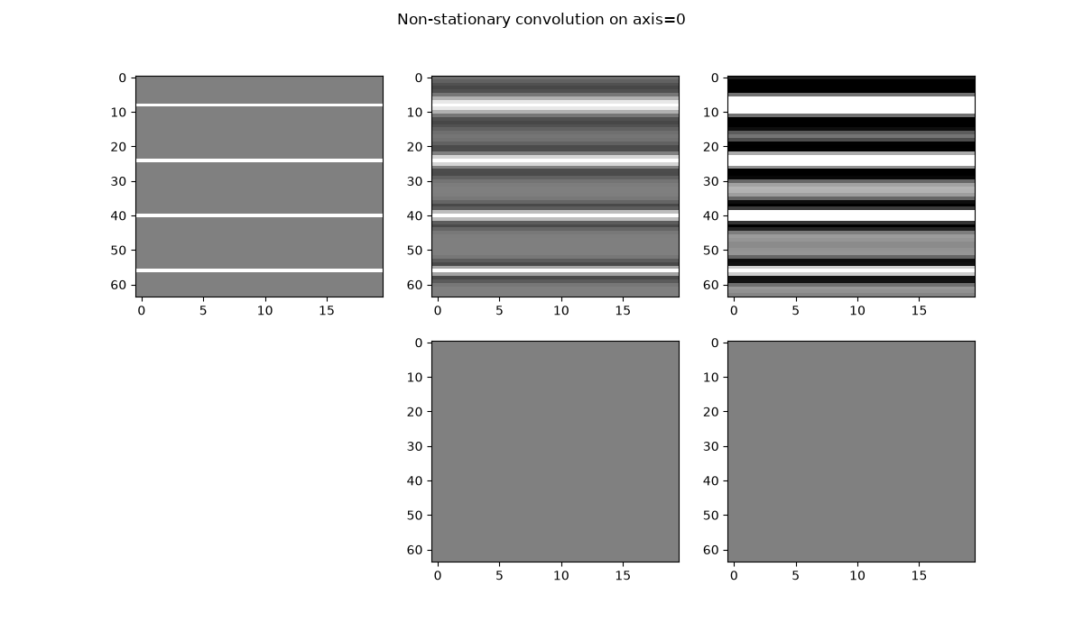
Whilst, up until now we can considered 1D signals, pylops.signalprocessing.NonStationaryConvolve1D can also operate on NDarray, applying non-stationary filters over one axis. Let’s consider here a 2D signal with the filters applied over the first axis.

# Input signal
t = np.arange(n) * dt
x = np.zeros((n, 20), dtype=np.float64)
x[ih] = 1.0

# Distributed array
x_dist = pylops_mpi.DistributedArray(
    global_shape=n * 20,
    base_comm=comm,
    partition=pylops_mpi.Partition.SCATTER)
x_dist.local_array[:] = x[nlocal * rank: nlocal * (rank + 1)].ravel()

# Create operator
COp_dist = pylops_mpi.signalprocessing.MPINonStationaryConvolve1D(
    (n, 20), wavs, ih, axis=0, base_comm=comm)

# Apply operator
y_dist = COp_dist @ x_dist
xadj_dist = COp_dist.H @ y_dist

y_dist = y_dist.asarray().reshape(n, 20)
xadj_dist = xadj_dist.asarray().reshape(n, 20)

# Create and apply benchmark serial operator
COp = pylops.signalprocessing.NonStationaryConvolve1D(
    dims=(n, 20), hs=wavs, ih=ih, axis=0,
)

y = COp @ x
xadj = COp.H @ y

if rank == 0:
    fig, axs = plt.subplots(2, 3, figsize=(12, 7))
    fig.suptitle("Non-stationary convolution on axis=0")
    axs[0][0].imshow(x, cmap="gray", vmin=-1, vmax=1)
    axs[0][1].imshow(y_dist, cmap="gray", vmin=-1, vmax=1)
    axs[0][2].imshow(xadj_dist, cmap="gray", vmin=-1, vmax=1)
    axs[1][0].axis("off")
    axs[1][1].imshow(y_dist - y, cmap="gray", vmin=-1, vmax=1)
    axs[1][2].imshow(xadj_dist - xadj, cmap="gray", vmin=-1, vmax=1)
    for ax in axs.ravel():
        ax.axis("tight")

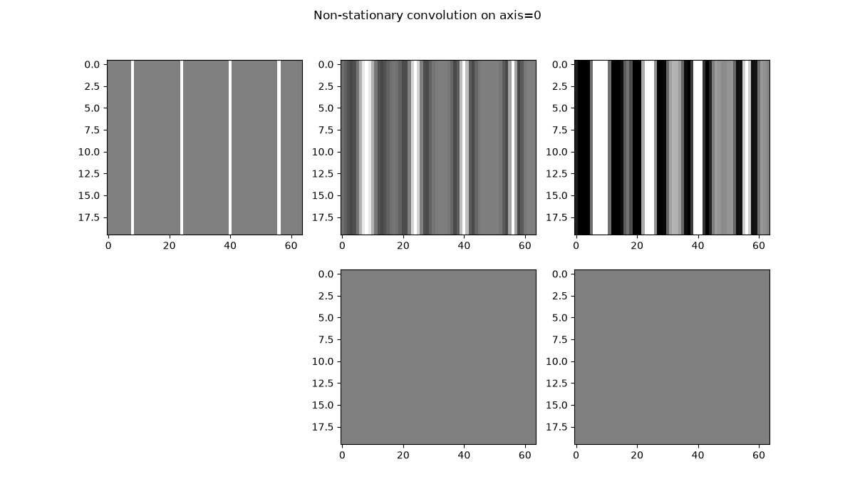
And on 2D signal with the filters applied over the second axis.

# Input signal
t = np.arange(n) * dt
x = np.zeros((20, n), dtype=np.float64)
x[:, ih] = 1.0

# Distributed array
x_dist = pylops_mpi.DistributedArray(
    global_shape=n * 20,
    base_comm=comm,
    partition=pylops_mpi.Partition.SCATTER)
x_dist.local_array[:] = x[:, nlocal * rank: nlocal * (rank + 1)].ravel()

# Create operator
COp_dist = pylops_mpi.signalprocessing.MPINonStationaryConvolve1D(
    (20, n), wavs, ih, axis=-1, base_comm=comm)

# Apply operator
y_dist = COp_dist @ x_dist
xadj_dist = COp_dist.H @ y_dist

y_dist = y_dist.asarray()
xadj_dist = xadj_dist.asarray()

y_dist = y_dist.reshape(size, 20, nlocal).transpose(1, 0, 2).reshape(20, -1)
xadj_dist = xadj_dist.reshape(size, 20, nlocal).transpose(1, 0, 2).reshape(20, -1)

# Create and apply benchmark serial operator
COp = pylops.signalprocessing.NonStationaryConvolve1D(
    (20, n), wavs, ih, axis=-1,
)

y = COp @ x
xadj = COp.H @ y

if rank == 0:
    fig, axs = plt.subplots(2, 3, figsize=(12, 7))
    fig.suptitle("Non-stationary convolution on axis=0")
    axs[0][0].imshow(x, cmap="gray", vmin=-1, vmax=1)
    axs[0][1].imshow(y_dist, cmap="gray", vmin=-1, vmax=1)
    axs[0][2].imshow(xadj_dist, cmap="gray", vmin=-1, vmax=1)
    axs[1][0].axis("off")
    axs[1][1].imshow(y_dist - y, cmap="gray", vmin=-1, vmax=1)
    axs[1][2].imshow(xadj_dist - xadj, cmap="gray", vmin=-1, vmax=1)
    for ax in axs.ravel():
        ax.axis("tight")