6. Multiscale Local Directions

This example shows how to use the Curvelet transform to visualize local, multiscale preferrential directions in an image. Inspired by Kymatio’s Scattering disks.

# sphinx_gallery_thumbnail_number = 3

import matplotlib as mpl
import matplotlib.pyplot as plt
import numpy as np
import numpy.typing as npt
from mpl_toolkits.axes_grid1 import make_axes_locatable
from pylops.signalprocessing import FFT2D

from curvelops import FDCT2D
from curvelops.plot import (
    create_axes_grid,
    create_inset_axes_grid,
    overlay_arrows,
    overlay_disks,
)
from curvelops.utils import array_split_nd, ndargmax

Input

inputfile = "../testdata/sigmoid.npz"

data = np.load(inputfile)
data = data["sigmoid"]
nx, nz = data.shape
dx, dz = 0.005, 0.004
x, z = np.arange(nx) * dx, np.arange(nz) * dz

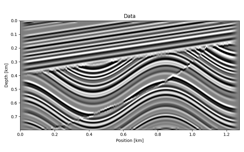
aspect = dz / dx
figsize_aspect = aspect * nz / nx
opts_space = dict(
    extent=(x[0], x[-1], z[-1], z[0]),
    cmap="gray",
    interpolation="lanczos",
    aspect=aspect,
)
vmax = 0.5 * np.max(np.abs(data))
fig, ax = plt.subplots(figsize=(8, figsize_aspect * 8))
ax.imshow(data.T, vmin=-vmax, vmax=vmax, **opts_space)
ax.set(xlabel="Position [km]", ylabel="Depth [km]", title="Data")
fig.tight_layout()

Understanding Curvelet Disks

First we create and apply curvelet transform.

Cop = FDCT2D(data.shape, nbscales=4, nbangles_coarse=8, allcurvelets=False)
d_c = Cop.struct(Cop @ data)

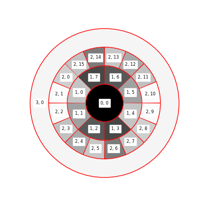
Each wedge is mapped to a region of the scattering disk. The first number refers to the scale, the second to the wedge index, zero-indexed.

The disks have the most energy in the direction perpendicular to the directions of minimum change. The following disk is computed with the entire image. We observe that with energy mostly along the top-bottom direction, the directions in the image will be mostly along the left-right direction, which matches the input data.

rows, cols = 1, 1
fig, axes = create_axes_grid(
    rows,
    cols,
    kwargs_subplots=dict(projection="polar"),
    kwargs_figure=dict(figsize=(4, 4)),
)
overlay_disks(d_c, axes, annotate=True)

Multiscale Local Directions

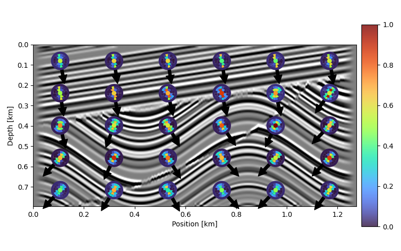
The power of the curvelet transform is to provide dip information varying with location and scale. Below we will compute preferrential local directions using an approach based on the 2D FFT that does not differentiate between scales.

rows, cols = 5, 6


def local_single_scale_dips(data: npt.NDArray, rows: int, cols: int) -> npt.NDArray:
    kvecs = np.empty((rows, cols, 2))
    d_split = array_split_nd(data.T, rows, cols)

    for irow in range(kvecs.shape[0]):
        for icol in range(kvecs.shape[1]):
            d_loc = d_split[irow][icol].T
            Fop_loc = FFT2D(
                d_loc.shape,
                sampling=[dx, dz],
                norm="ortho",
                real=False,
                ifftshift_before=True,
                fftshift_after=True,
                engine="scipy",
            )
            d_k_loc = Fop_loc @ d_loc

            kx_loc = Fop_loc.f1
            kz_loc = Fop_loc.f2

            kx_locmax, kz_locmax = ndargmax(np.abs(d_k_loc[:, kz_loc > 0]))

            k = np.array([kx_loc[kx_locmax], kz_loc[kz_loc > 0][kz_locmax]])
            kvecs[irow, icol, :] = k / np.linalg.norm(k)
    return kvecs

diskcmap = "turbo"
rows, cols = 5, 6
kvecs = local_single_scale_dips(data, rows, cols)
kvecs *= 0.15 * min(x[-1] - x[0], z[-1] - z[0])

fig, ax = plt.subplots(figsize=(8, figsize_aspect * 8))
ax.imshow(data.T, vmin=-vmax, vmax=vmax, **opts_space)
ax.set(xlabel="Position [km]", ylabel="Depth [km]")
divider = make_axes_locatable(ax)
cax = divider.append_axes("right", size="5%", pad=0.1)
mpl.colorbar.ColorbarBase(
    cax,
    cmap=plt.get_cmap(diskcmap),
    norm=mpl.colors.Normalize(vmin=0, vmax=1),
    alpha=0.8,
)

# Local single-scale directions
overlay_arrows(kvecs, ax)

# Local multsicale directions
axesin = create_inset_axes_grid(
    ax,
    rows,
    cols,
    height=0.6,
    width=0.6,
    kwargs_inset_axes=dict(projection="polar"),
)
overlay_disks(d_c, axesin, linewidth=0.0, cmap=diskcmap)
fig.tight_layout()