3. Visualizing Curvelet Coefficients

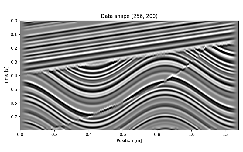
This example shows the how to visualize curvelet coefficients of an image, using as example a typical subsurface structure.

# sphinx_gallery_thumbnail_number = 3

import matplotlib.pyplot as plt
import numpy as np

from curvelops import FDCT2D, apply_along_wedges, curveshow

Input data

inputfile = "../testdata/sigmoid.npz"

d = np.load(inputfile)
d = d["sigmoid"]
nx, nt = d.shape
dx, dt = 0.005, 0.004
x, t = np.arange(nx) * dx, np.arange(nt) * dt

aspect = dt / dx
opts_plot = dict(
    extent=(x[0], x[-1], t[-1], t[0]),
    cmap="gray",
    interpolation="lanczos",
    aspect=aspect,
)
vmax = 0.5 * np.max(np.abs(d))
figsize_aspect = aspect * nt / nx
fig, ax = plt.subplots(figsize=(8, figsize_aspect * 8), sharey=True, sharex=True)
ax.imshow(d.T, vmin=-vmax, vmax=vmax, **opts_plot)
ax.set(xlabel="Position [m]", ylabel="Time [s]", title=f"Data shape {d.shape}")
fig.tight_layout()

Create Curvelet Transform

nbscales = 4
nbangles_coarse = 8
allcurvelets = False  # Last scale will be a wavelet transform

Cop = FDCT2D(
    d.shape,
    nbscales=nbscales,
    nbangles_coarse=nbangles_coarse,
    allcurvelets=allcurvelets,
)

Convert to a list of lists of ndarrays.

d_fdct_struct = Cop.struct(Cop @ d)

Real part of FDCT coefficients

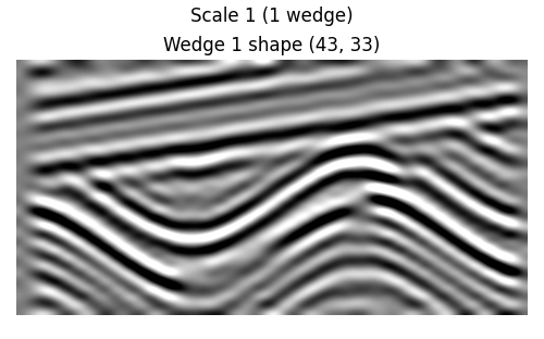
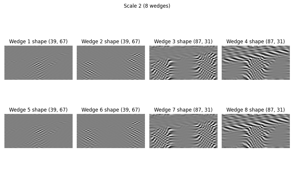
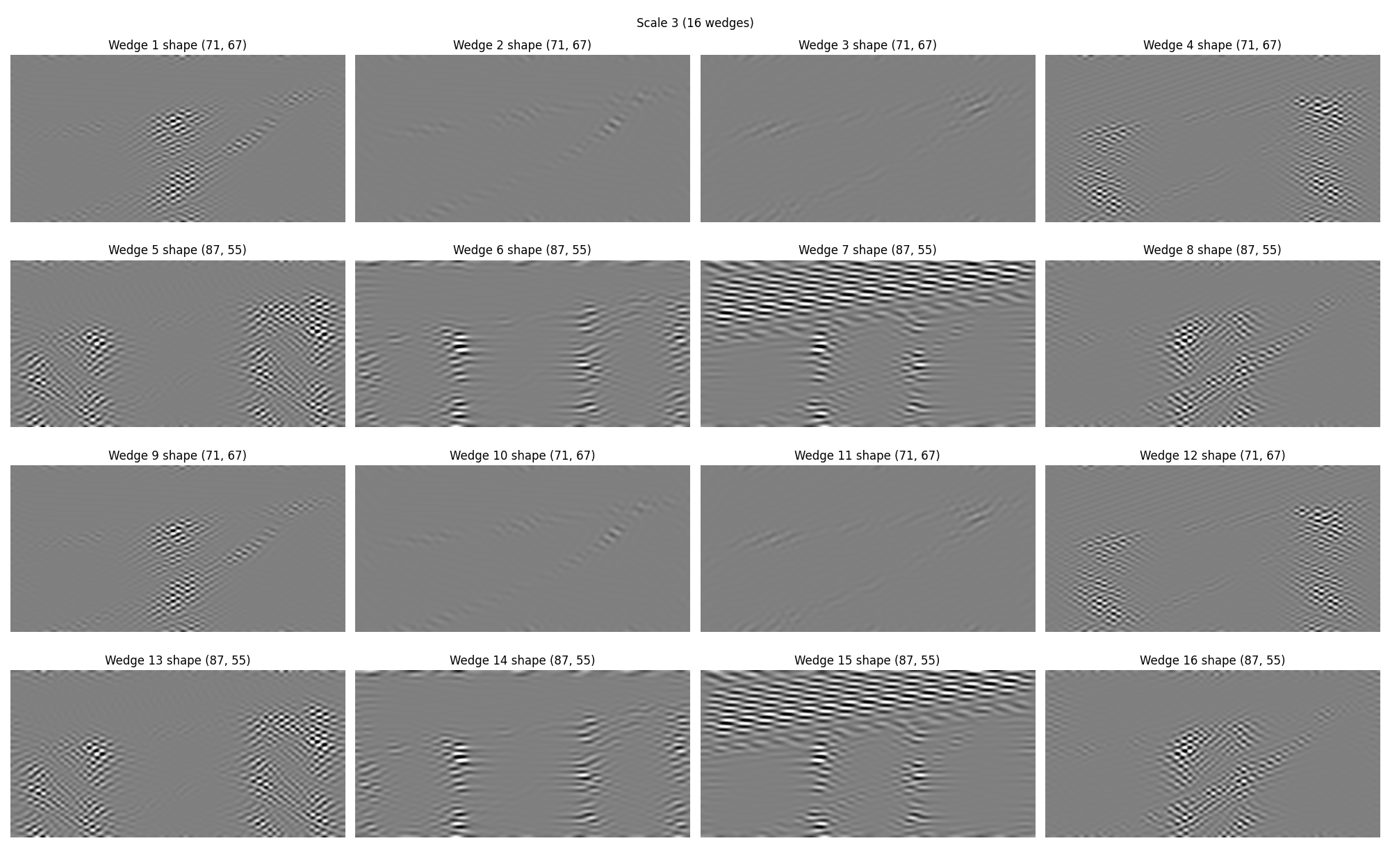
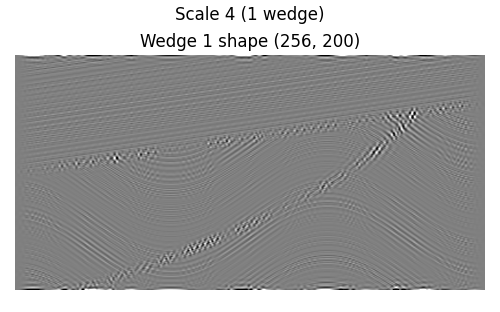
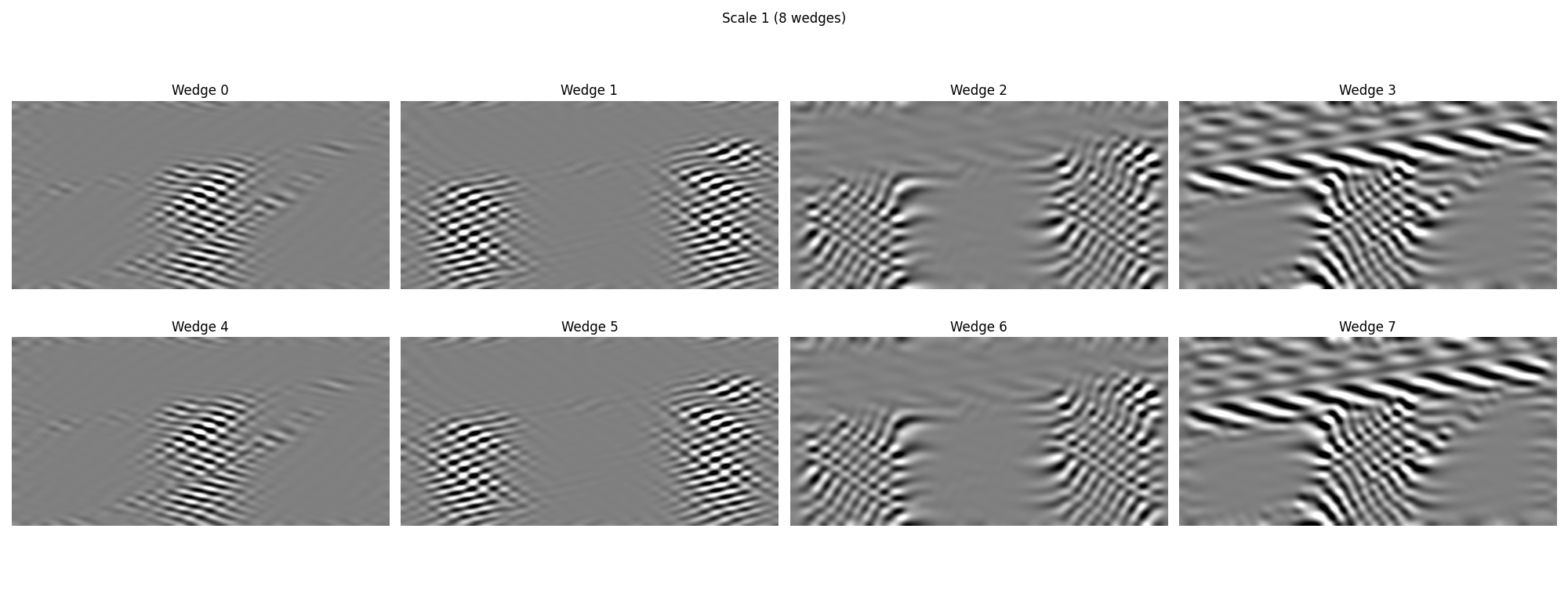
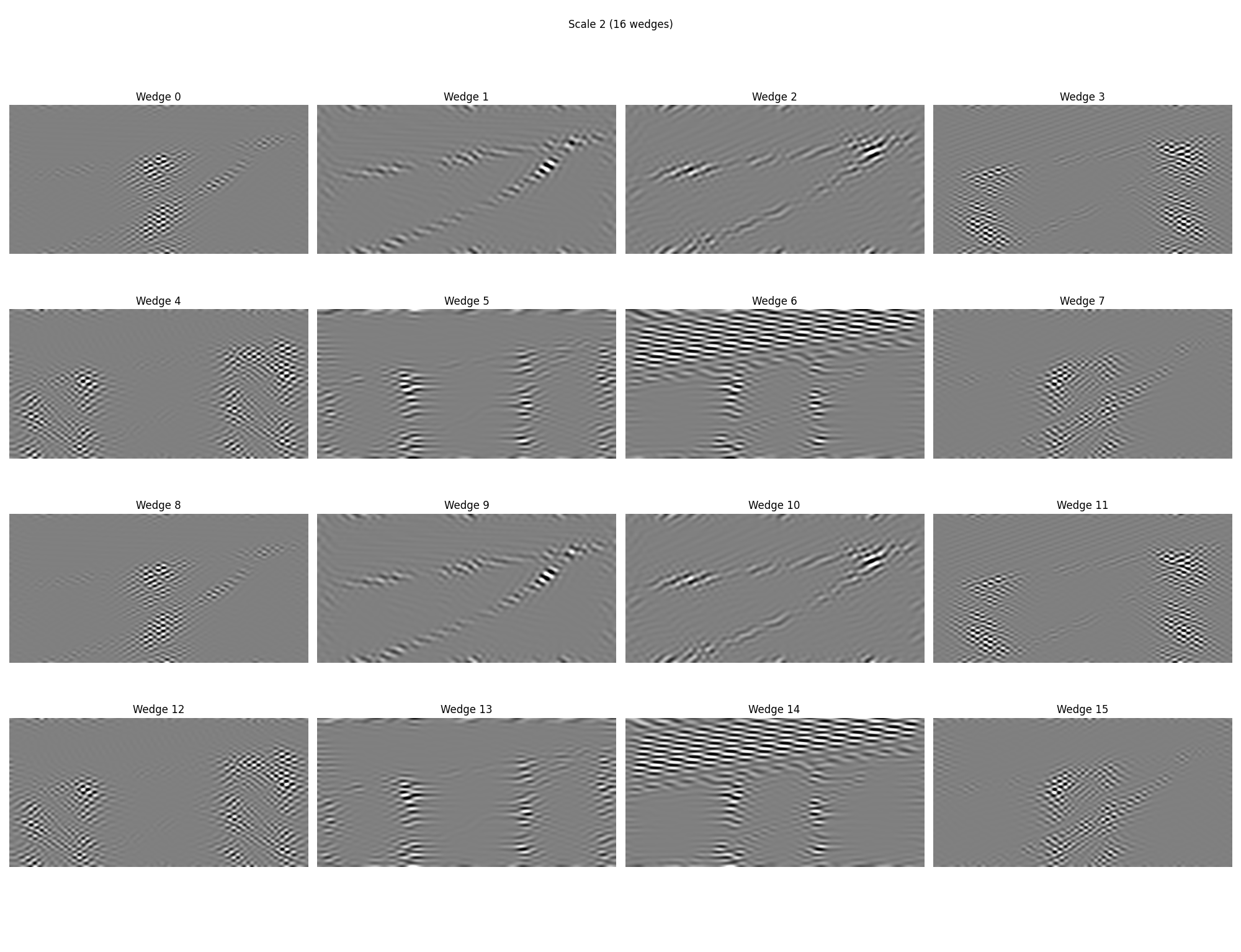
Curvelet coefficients are essentially directionally-filtered, shrunk versions of the original signal. Note that the “shrinking” does not preserve aspect ratio.

for j, c_scale in enumerate(d_fdct_struct, start=1):
    nangles = len(c_scale)
    rows = int(np.floor(np.sqrt(nangles)))
    cols = int(np.ceil(nangles / rows))
    fig, axes = plt.subplots(
        rows,
        cols,
        figsize=(5 * rows, figsize_aspect * 5 * rows),
    )
    fig.suptitle(f"Scale {j} ({len(c_scale)} wedge{'s' if len(c_scale) > 1 else ''})")
    axes = np.atleast_1d(axes).ravel()
    vmax = 0.5 * max(np.abs(Cweg).max() for Cweg in c_scale)
    for iw, (fdct_wedge, ax) in enumerate(zip(c_scale, axes), start=1):
        # Note that wedges are transposed in comparison to the input vector.
        # This is due to the underlying implementation of the transform. In
        # order to plot in the same manner as the data, we must first
        # transpose the wedge. We will using the transpose of the wedge for
        # visualization.
        c = fdct_wedge.real.T
        ax.imshow(c.T, vmin=-vmax, vmax=vmax, **opts_plot)
        ax.set(title=f"Wedge {iw} shape {c.shape}")
        ax.axis("off")
    fig.tight_layout()

• 
• 
• 
• 

Imaginagy part of FDCT coefficients

Curvelops includes much of the above logic wrapped in the following curvelops.plot.cuveshow. Since we

# Normalize each coefficient by max abs
y_norm = apply_along_wedges(d_fdct_struct, lambda w, *_: w / np.abs(w).max())

figs = curveshow(
    y_norm,
    real=False,
    kwargs_imshow={**opts_plot, "vmin": -0.5, "vmax": 0.5},
)

• 
• 
• 
•