Seismic pre-stack inversion

Estimation of the elastic parameters of the subsurface (P-wave velocity, S-wave velocity and density) from band-limited pre-stack seismic data (angle gathers), using their amplitude variation with angle (AVO).

• True model: the logarithm of the elastic parameters, \(\mathbf{m} = [\ln V_P, \ln V_S, \ln \rho]\), stacked along the second axis.

• Operator: pylops.avo.prestack.PrestackLinearModelling, a first derivative along depth, followed by the Aki-Richards linearization of the AVO response and a convolution with the wavelet, \(d(t, \theta) = w(t) * \sum_{i=1}^{3} G_i(t, \theta) \frac{\mathrm{d} \ln m_i(t)}{\mathrm{d} t}\), applied to every trace.

• Data: the pre-stack seismic data, plus white Gaussian noise (noise_std, drawn with a fixed seed).

The wavelet, the angles and a smooth background model are given to the solvers, which use the latter as starting guess. The three parameters have different sensitivities to the data, so every solver weights its regularization (or damping) separately for \(V_P\), \(V_S\) and \(\rho\) (parameters with suffixes _vp, _vs and _rho).

Solvers compared:

Solver	Formulation
LSTSQ-TraceByTrace	Damped least squares solved independently for each trace through the normal equations, with a direct solver
LSQR-Laplacian	Regularized least squares with a 2D Laplacian (smoothness) regularizer on each parameter, solved with LSQR starting from the trace-by-trace solution
SplitBregman-Blocky	Blockiness-promoting inversion with L1 on the first derivative along depth and L2 on the second derivative along space of each parameter, solved with Split Bregman
LinearizedADMM-TV	Isotropic total variation regularization of each parameter, solved with linearized ADMM (PyProximal), starting from the trace-by-trace solution
ADMML2-TV	Isotropic total variation regularization of each parameter, solved with ADMM specialized for an L2 misfit (PyProximal), starting from the trace-by-trace solution
PrimalDual-TV	Isotropic total variation regularization of each parameter, solved with the primal-dual algorithm (PyProximal), starting from the trace-by-trace solution

All total variation solvers use forward differences along depth and space (never across parameters).

Source: benchmarks/seismic_prestack.

Results

Raw results: results/seismic_prestack.csv.

Marmousi

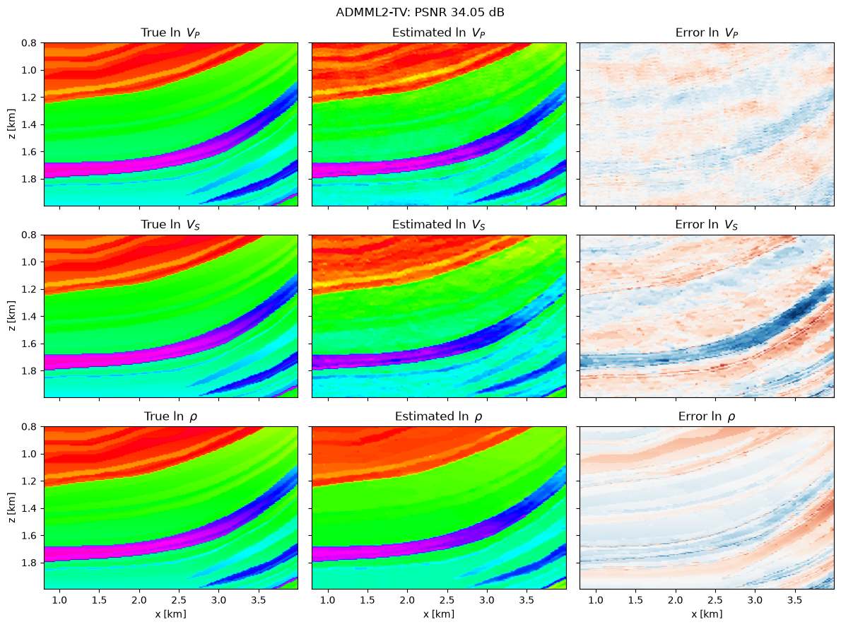
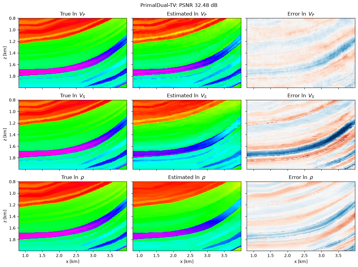
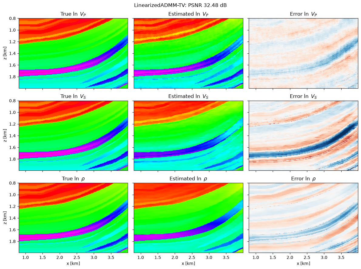
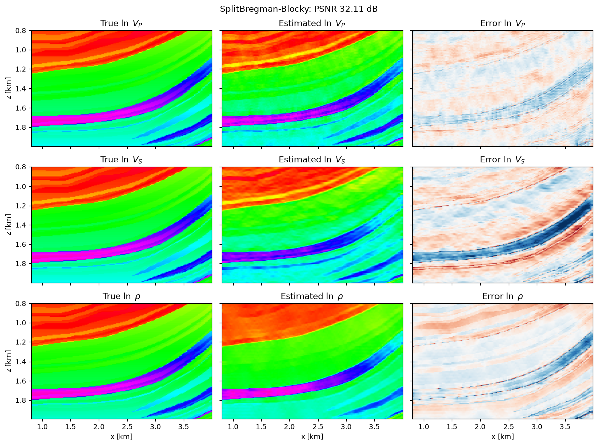
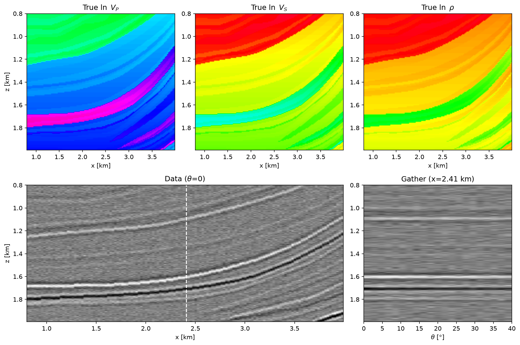
2D section of a Marmousi-like elastic model, plus white Gaussian noise.

The P-wave velocity is the acoustic impedance of the PyLops poststack_model (first 300 depth samples, one every six traces) taken as velocity in m/s, the S-wave velocity is half of it and the density is \(\rho = V_P / 3 + 300\). The model is the logarithm of the three parameters, with 300 depth samples, 3 parameters and 134 traces (4 m and 24 m spacing). Data are modelled with the Aki-Richards linearization (\(V_S/V_P = 0.5\)), 21 angles between 0° and 40° and a 15 Hz Ricker wavelet of 41 samples (4 ms sampling). The background model, used by the solvers as starting guess, is the true model smoothed with a moving average of 30 samples in depth and 25 in space.

Dataset parameters: noise_std=0.05, seed=10

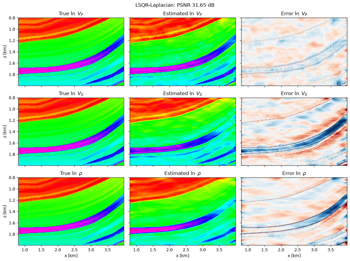
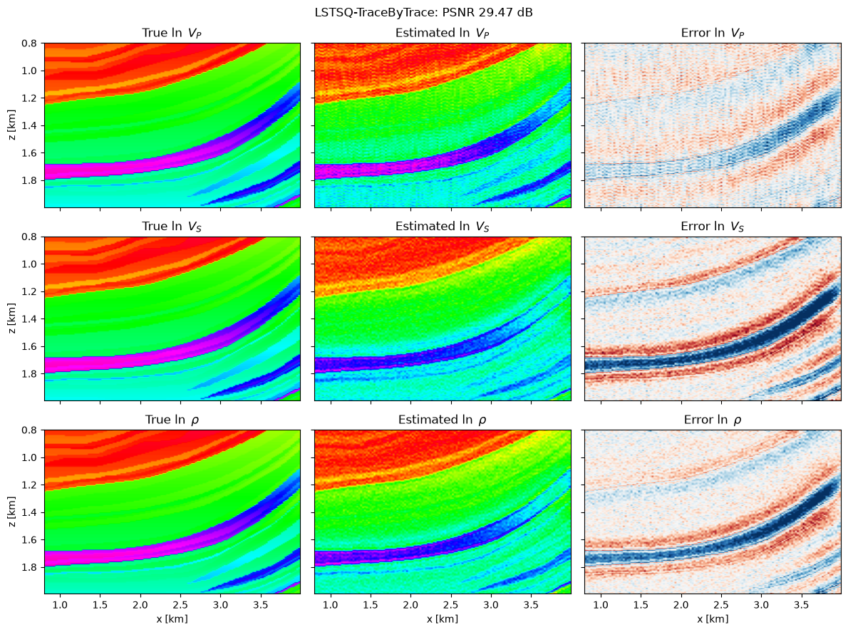
Rank	Solver	MAE	PSNR [dB]	Time [s]	Figure
1	ADMML2-TV	0.02277	34.05	37.095	view
2	PrimalDual-TV	0.02635	32.48	68.288	view
3	LinearizedADMM-TV	0.02635	32.48	75.596	view
4	SplitBregman-Blocky	0.02779	32.11	70.396	view
5	LSQR-Laplacian	0.02929	31.65	33.680	view
6	LSTSQ-TraceByTrace	0.03835	29.47	0.267	view