Seismic post-stack inversion

Estimation of the acoustic impedance of the subsurface from band-limited post-stack seismic data.

• True model: the logarithm of the acoustic impedance, \(\ln \text{AI}\).

• Operator: pylops.avo.poststack.PoststackLinearModelling, a first derivative along depth followed by a convolution with the wavelet, \(d = \frac{1}{2} w * \frac{\mathrm{d} \ln \text{AI}}{\mathrm{d} z}\), applied to every trace.

• Data: the post-stack seismic data, plus white Gaussian noise (noise_std, drawn with a fixed seed).

The wavelet and a smooth background model are given to the solvers, which use the latter as starting guess.

Solvers compared:

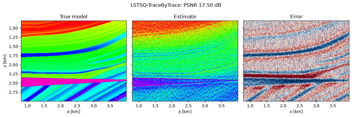
Solver	Formulation
LSTSQ-TraceByTrace	Damped least squares solved independently for each trace through the normal equations, with a direct solver
LSQR-Laplacian	Regularized least squares with a 2D Laplacian (smoothness) regularizer, solved with LSQR starting from the trace-by-trace solution
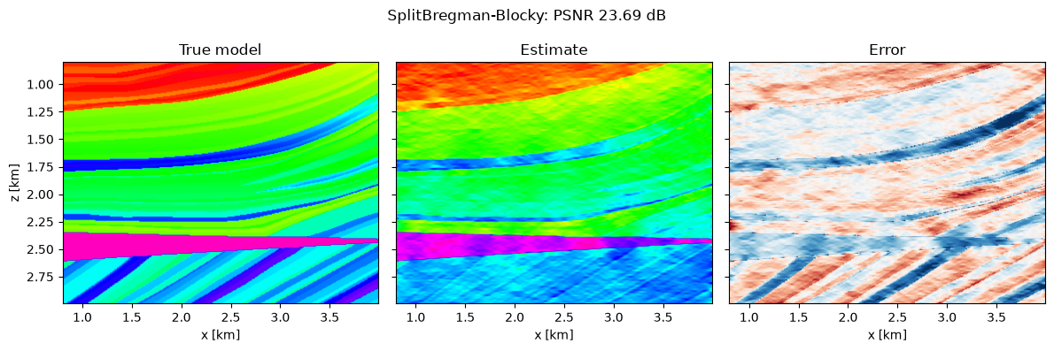
SplitBregman-Blocky	Blockiness-promoting inversion with L1 on the first derivative along depth and L2 on the second derivative along space, solved with Split Bregman
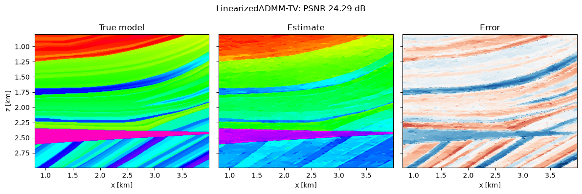
LinearizedADMM-TV	Isotropic total variation regularization, solved with linearized ADMM (PyProximal)
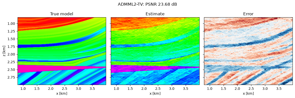
ADMML2-TV	Isotropic total variation regularization, solved with ADMM specialized for an L2 misfit (PyProximal)
ADMM-TV	Total variation regularization, solved with ADMM with an iterative TV proximal operator (PyProximal)
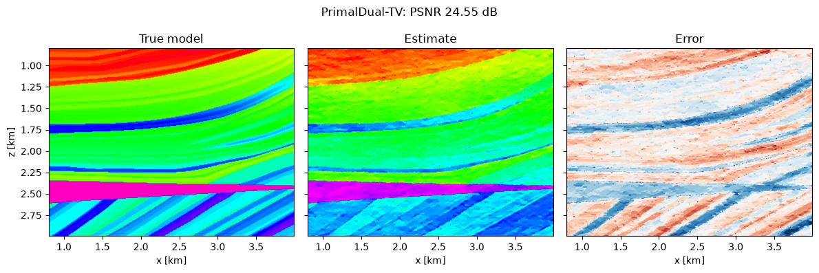
PrimalDual-TV	Isotropic total variation regularization, solved with the primal-dual algorithm (PyProximal)
PnP-ADMM-BM3D	Plug-and-Play prior with the BM3D denoiser in place of the proximal operator of the regularizer, solved with ADMM (PyProximal)
RED-BM3D	Regularization by Denoising with the BM3D denoiser, solved with fixed-point iterations (PyProximal)

All total variation solvers use pylops.Gradient with forward differences.

Source: benchmarks/seismic_poststack.

Results

Raw results: results/seismic_poststack.csv.

Marmousi

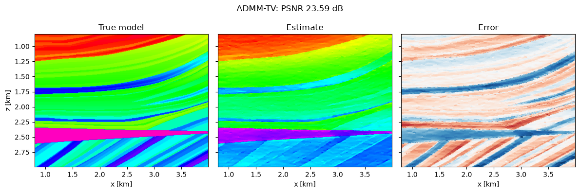
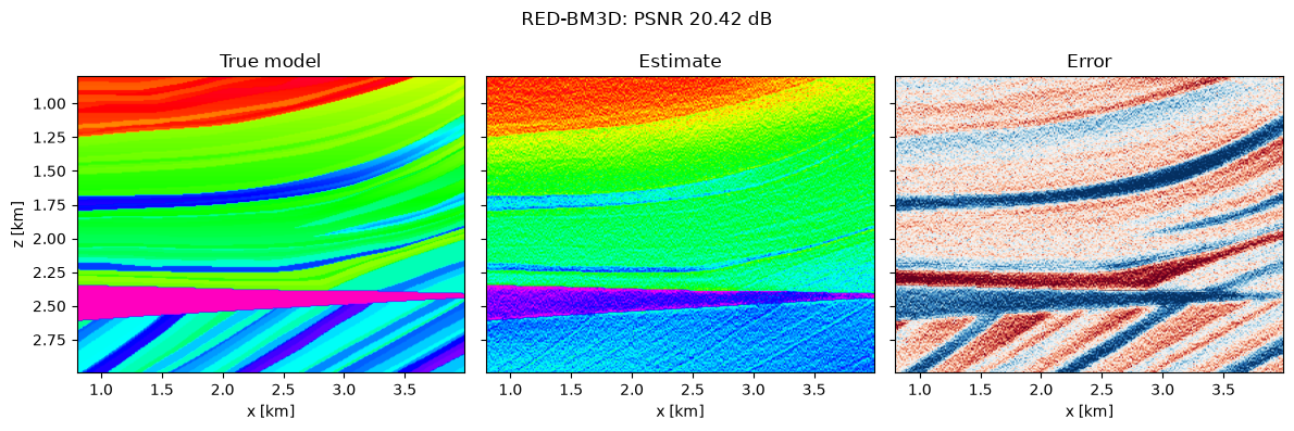
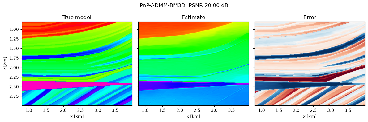
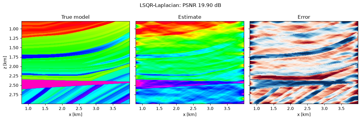
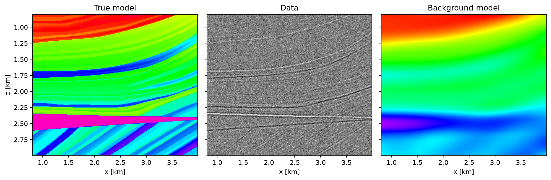
2D section of a Marmousi-like acoustic impedance model, plus white Gaussian noise.

The model is the logarithm of the acoustic impedance of the PyLops poststack_model (one every three traces), with 550 depth samples and 267 traces (4 m and 12 m spacing). Data are modelled with a 20 Hz Ricker wavelet of 41 samples (4 ms sampling). The background model, used by the solvers as starting guess, is the true model smoothed with a moving average of 60 samples in depth and 50 in space.

Dataset parameters: noise_std=0.1, seed=10

Rank	Solver	MAE	PSNR [dB]	Time [s]	Figure
1	PrimalDual-TV	0.05332	24.55	25.937	view
2	LinearizedADMM-TV	0.05408	24.29	26.785	view
3	SplitBregman-Blocky	0.05806	23.69	31.484	view
4	ADMML2-TV	0.05944	23.68	32.836	view
5	ADMM-TV	0.05892	23.59	31.583	view
6	RED-BM3D	0.08493	20.42	56.175	view
7	PnP-ADMM-BM3D	0.08375	20.00	56.714	view
8	LSQR-Laplacian	0.09039	19.90	13.816	view
9	LSTSQ-TraceByTrace	0.1199	17.50	0.131	view