

Note
Go to the end to download the full example code.
Post Stack Inversion - 3D#
This tutorial demonstrates the implementation of a distributed 3D Post-stack inversion. It consists of a first part showing how to model a 3D synthetic post-stack seismic data from a 3D model of the subsurface acoustic impedance in a distributed manner, following by a second part when inversion is carried out.
This tutorial builds on the pylops.avo.poststack.PoststackLinearModelling
operator to model 1d post-stack seismic traces 1d profiles of the subsurface acoustic impedence
by means of the following equation
where \(\text{AI}(t)\) is the acoustic impedance profile and \(w(t)\) is the time domain seismic wavelet. Being this inherently a 1d operator, we can easily set up a problem where one of the dimensions (here the y-dimension) is distributed across ranks and each of them is in charge of performing modelling for a subvolume of the entire domain. Using a compact matrix-vector notation, the entire problem can be written as
where \(\mathbf{G}_i\) is a post-stack modelling operator, \(\mathbf{d}_i\) is the data, and \(\mathbf{ai}_i\) is the input model for the i-th portion of the model.
This problem can be easily set up using the pylops_mpi.basicoperators.MPIBlockDiag
operator.
import numpy as np
from scipy.signal import filtfilt
from matplotlib import pyplot as plt
from mpi4py import MPI

from pylops.utils.wavelets import ricker
from pylops.basicoperators import Transpose
from pylops.avo.poststack import PoststackLinearModelling

import pylops_mpi

plt.close("all")
rank = MPI.COMM_WORLD.Get_rank()
size = MPI.COMM_WORLD.Get_size()
Let’s start by defining all the parameters required by the
pylops.avo.poststack.PoststackLinearModelling operator.
# Model
model = np.load("../testdata/avo/poststack_model.npz")
x, z, m = model['x'][::3], model['z'], np.log(model['model'])[:, ::3]

# Making m a 3D model
ny_i = 20  # size of model in y direction for rank i
y = np.arange(ny_i)
m3d_i = np.tile(m[:, :, np.newaxis], (1, 1, ny_i)).transpose((2, 1, 0))
ny_i, nx, nz = m3d_i.shape

# Size of y at all ranks
ny = MPI.COMM_WORLD.allreduce(ny_i)

# Smooth model
nsmoothy, nsmoothx, nsmoothz = 5, 30, 20
mback3d_i = filtfilt(np.ones(nsmoothy) / float(nsmoothy), 1, m3d_i, axis=0)
mback3d_i = filtfilt(np.ones(nsmoothx) / float(nsmoothx), 1, mback3d_i, axis=1)
mback3d_i = filtfilt(np.ones(nsmoothz) / float(nsmoothz), 1, mback3d_i, axis=2)

# Wavelet
dt = 0.004
t0 = np.arange(nz) * dt
ntwav = 41
wav = ricker(t0[:ntwav // 2 + 1], 15)[0]

# Collecting all the m3d and mback3d at all ranks
m3d = np.concatenate(MPI.COMM_WORLD.allgather(m3d_i))
mback3d = np.concatenate(MPI.COMM_WORLD.allgather(mback3d_i))
We now create the linear operator version of
pylops.avo.poststack.PoststackLinearModelling at each rank to model a
subset of the data along the y-axis. Such operators are passed
to the pylops_mpi.basicoperators.MPIBlockDiag operator, which is then used to perform
the different forward operations of each individual operator
at different ranks to compute the overall data. Note that to simplify the
handling of the model and data, we split and distribute the first axis,
and use pylops.Transpose to rearrange the model and data
in the form required by the pylops.avo.poststack.PoststackLinearModelling
operator.
# Create flattened model data
m3d_dist = pylops_mpi.DistributedArray(global_shape=ny * nx * nz)
m3d_dist[:] = m3d_i.flatten()

# Create flattened smooth model data
mback3d_dist = pylops_mpi.DistributedArray(global_shape=ny * nx * nz)
mback3d_dist[:] = mback3d_i.flatten()

# LinearOperator PostStackLinearModelling
PPop = PoststackLinearModelling(wav, nt0=nz, spatdims=(ny_i, nx))
Top = Transpose((ny_i, nx, nz), (2, 0, 1))
BDiag = pylops_mpi.basicoperators.MPIBlockDiag(ops=[Top.H @ PPop @ Top, ])

# Data
d_dist = BDiag @ m3d_dist
d_local = d_dist.local_array.reshape((ny_i, nx, nz))
d = d_dist.asarray().reshape((ny, nx, nz))
d_0_dist = BDiag @ mback3d_dist
d_0 = d_dist.asarray().reshape((ny, nx, nz))
We perform 2 different kinds of inversions:
Inversion calculated iteratively using the
pylops_mpi.optimization.cls_basic.CGLSsolver.Inversion with spatial regularization using normal equations along all three dimensions (x, y and z). This requires extending the operator and data in the following manner:
where \(\mathbf{L}\) is the pylops_mpi.basicoperators.MPILaplacian operator
which is used to apply second derivative along all three axes, \(\mathbf{N}\) is an operator computing the
normal equations, and \(\mathbf{d}^{Norm}\) is the data of the normal equation operator used for inversion.
# Inversion using CGLS solver
minv3d_iter_dist = pylops_mpi.optimization.basic.cgls(BDiag, d_dist, x0=mback3d_dist, niter=100, show=True)[0]
minv3d_iter = minv3d_iter_dist.asarray().reshape((ny, nx, nz))
CGLS
-----------------------------------------------------------------
The Operator Op has 2937000 rows and 2937000 cols
damp = 0.000000e+00     tol = 1.000000e-04      niter = 100
-----------------------------------------------------------------

    Itn          x[0]              r1norm         r2norm
     1        6.2034e-01         7.5690e+01     7.5690e+01
     2        6.2500e-01         4.5718e+01     4.5718e+01
     3        6.2669e-01         3.3126e+01     3.3126e+01
     4        6.2452e-01         2.6621e+01     2.6621e+01
     5        6.2091e-01         2.2097e+01     2.2097e+01
     6        6.1845e-01         1.8653e+01     1.8653e+01
     7        6.1636e-01         1.5872e+01     1.5872e+01
     8        6.1486e-01         1.3797e+01     1.3797e+01
     9        6.1562e-01         1.2071e+01     1.2071e+01
    10        6.1730e-01         1.0660e+01     1.0660e+01
    11        6.1619e-01         9.5376e+00     9.5376e+00
    21        6.1733e-01         4.7497e+00     4.7497e+00
    31        6.1264e-01         2.9346e+00     2.9346e+00
    41        6.1379e-01         2.0154e+00     2.0154e+00
    51        6.1548e-01         1.5044e+00     1.5044e+00
    61        6.1695e-01         1.1912e+00     1.1912e+00
    71        6.1561e-01         1.0001e+00     1.0001e+00
    81        6.1437e-01         8.6449e-01     8.6449e-01
    91        6.1327e-01         7.2838e-01     7.2838e-01
    92        6.1343e-01         7.1870e-01     7.1870e-01
    93        6.1361e-01         7.1127e-01     7.1127e-01
    94        6.1389e-01         7.0269e-01     7.0269e-01
    95        6.1422e-01         6.9241e-01     6.9241e-01
    96        6.1453e-01         6.8123e-01     6.8123e-01
    97        6.1485e-01         6.7010e-01     6.7010e-01
    98        6.1520e-01         6.5942e-01     6.5942e-01
    99        6.1544e-01         6.5026e-01     6.5026e-01
   100        6.1561e-01         6.4212e-01     6.4212e-01

Iterations = 100        Total time (s) = 27.57
-----------------------------------------------------------------
# Regularized inversion with normal equations
epsR = 1e2
LapOp = pylops_mpi.MPILaplacian(dims=(ny, nx, nz), axes=(0, 1, 2), weights=(1, 1, 1),
                                sampling=(1, 1, 1), dtype=BDiag.dtype)
NormEqOp = BDiag.H @ BDiag + epsR * LapOp.H @ LapOp
dnorm_dist = BDiag.H @ d_dist
minv3d_ne_dist = pylops_mpi.optimization.basic.cg(NormEqOp, dnorm_dist, x0=mback3d_dist, niter=100, show=True)[0]
minv3d_ne = minv3d_ne_dist.asarray().reshape((ny, nx, nz))
CG
-------------------------------------------------------
The Operator Op has 2937000 rows and 2937000 cols
tol = 1.000000e-04      niter = 100
-------------------------------------------------------

    Itn           x[0]              r2norm
     1         6.1587e-01         1.6825e+03
     2         6.1667e-01         1.6533e+03
     3         6.1695e-01         1.4528e+03
     4         6.1725e-01         1.6359e+03
     5         6.1746e-01         1.3555e+03
     6         6.1767e-01         1.2633e+03
     7         6.1787e-01         1.3221e+03
     8         6.1811e-01         1.2846e+03
     9         6.1831e-01         1.1952e+03
    10         6.1851e-01         1.1626e+03
    11         6.1869e-01         1.1780e+03
    21         6.2050e-01         7.4711e+02
    31         6.2265e-01         6.6863e+02
    41         6.2516e-01         5.1781e+02
    51         6.2692e-01         4.3140e+02
    61         6.2847e-01         3.7187e+02
    71         6.2977e-01         2.9441e+02
    81         6.3072e-01         2.6242e+02
    91         6.3077e-01         2.3101e+02
    92         6.3075e-01         2.3022e+02
    93         6.3072e-01         2.2334e+02
    94         6.3068e-01         2.2033e+02
    95         6.3063e-01         2.1755e+02
    96         6.3056e-01         2.1555e+02
    97         6.3049e-01         2.1291e+02
    98         6.3041e-01         2.0469e+02
    99         6.3033e-01         1.9903e+02
   100         6.3026e-01         1.9777e+02

Iterations = 100        Total time (s) = 39.01
-------------------------------------------------------
# Regularized inversion with regularized equations
StackOp = pylops_mpi.MPIStackedVStack([BDiag, np.sqrt(epsR) * LapOp])
d0_dist = pylops_mpi.DistributedArray(global_shape=ny * nx * nz)
d0_dist[:] = 0.
dstack_dist = pylops_mpi.StackedDistributedArray([d_dist, d0_dist])

dnorm_dist = BDiag.H @ d_dist
minv3d_reg_dist = pylops_mpi.optimization.basic.cgls(
    StackOp, dstack_dist, x0=mback3d_dist, niter=100, show=False)[0]
minv3d_reg = minv3d_reg_dist.asarray().reshape((ny, nx, nz))
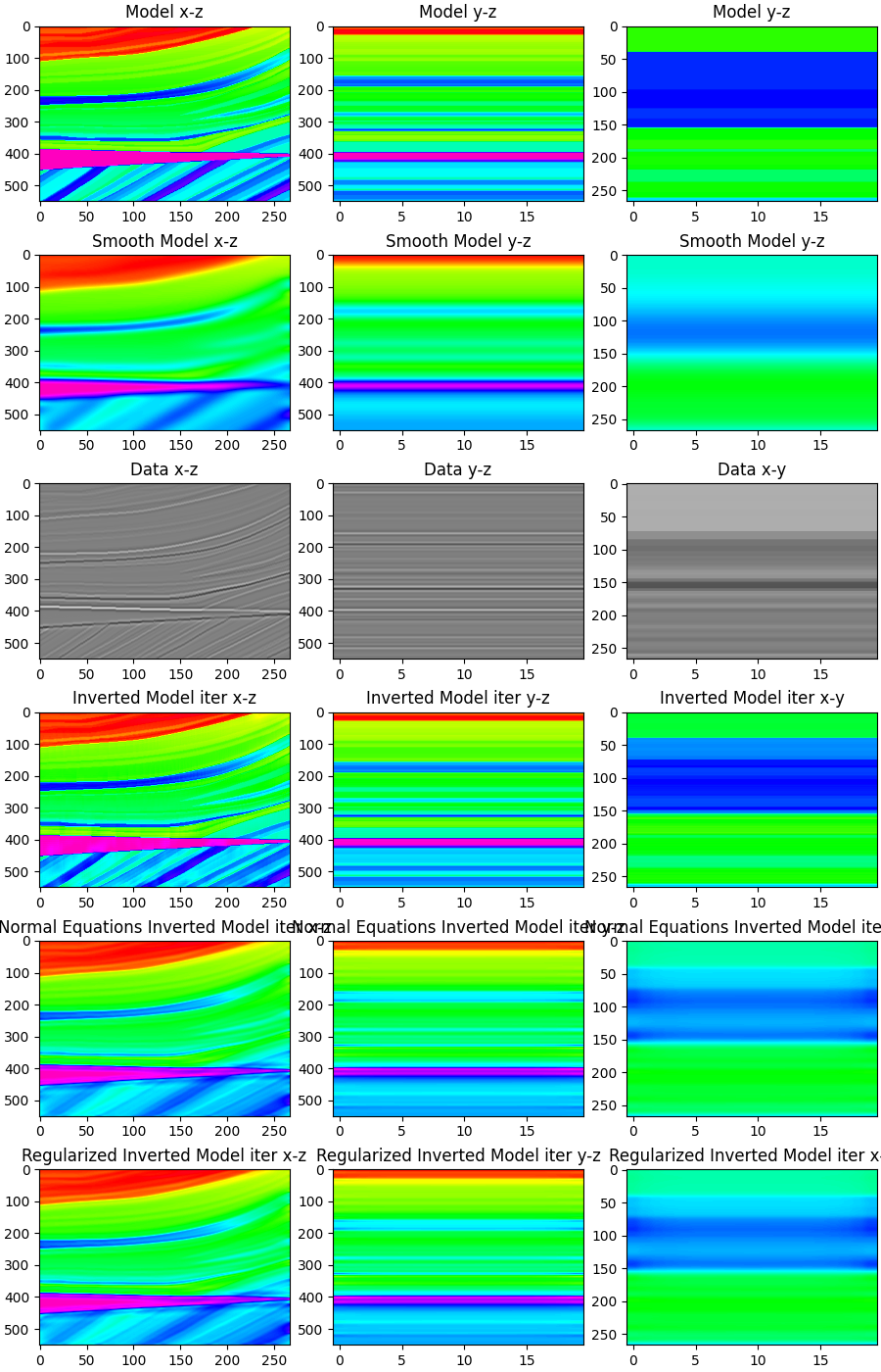
Finally, we display the modeling and inversion results
if rank == 0:
    # Check the distributed implementation gives the same result
    # as the one running only on rank0
    PPop0 = PoststackLinearModelling(wav, nt0=nz, spatdims=(ny, nx))
    d0 = (PPop0 @ m3d.transpose(2, 0, 1)).transpose(1, 2, 0)

    # Check the two distributed implementations give the same modelling results
    print('Distr == Local', np.allclose(d, d0))

    # Visualize
    fig, axs = plt.subplots(nrows=6, ncols=3, figsize=(9, 14), constrained_layout=True)
    axs[0][0].imshow(m3d[5, :, :].T, cmap="gist_rainbow", vmin=m.min(), vmax=m.max())
    axs[0][0].set_title("Model x-z")
    axs[0][0].axis("tight")
    axs[0][1].imshow(m3d[:, 200, :].T, cmap="gist_rainbow", vmin=m.min(), vmax=m.max())
    axs[0][1].set_title("Model y-z")
    axs[0][1].axis("tight")
    axs[0][2].imshow(m3d[:, :, 220].T, cmap="gist_rainbow", vmin=m.min(), vmax=m.max())
    axs[0][2].set_title("Model y-z")
    axs[0][2].axis("tight")

    axs[1][0].imshow(mback3d[5, :, :].T, cmap="gist_rainbow", vmin=m.min(), vmax=m.max())
    axs[1][0].set_title("Smooth Model x-z")
    axs[1][0].axis("tight")
    axs[1][1].imshow(mback3d[:, 200, :].T, cmap="gist_rainbow", vmin=m.min(), vmax=m.max())
    axs[1][1].set_title("Smooth Model y-z")
    axs[1][1].axis("tight")
    axs[1][2].imshow(mback3d[:, :, 220].T, cmap="gist_rainbow", vmin=m.min(), vmax=m.max())
    axs[1][2].set_title("Smooth Model y-z")
    axs[1][2].axis("tight")

    axs[2][0].imshow(d[5, :, :].T, cmap="gray", vmin=-1, vmax=1)
    axs[2][0].set_title("Data x-z")
    axs[2][0].axis("tight")
    axs[2][1].imshow(d[:, 200, :].T, cmap='gray', vmin=-1, vmax=1)
    axs[2][1].set_title('Data y-z')
    axs[2][1].axis('tight')
    axs[2][2].imshow(d[:, :, 220].T, cmap='gray', vmin=-1, vmax=1)
    axs[2][2].set_title('Data x-y')
    axs[2][2].axis('tight')

    axs[3][0].imshow(minv3d_iter[5, :, :].T, cmap="gist_rainbow", vmin=m.min(), vmax=m.max())
    axs[3][0].set_title("Inverted Model iter x-z")
    axs[3][0].axis("tight")
    axs[3][1].imshow(minv3d_iter[:, 200, :].T, cmap='gist_rainbow', vmin=m.min(), vmax=m.max())
    axs[3][1].set_title('Inverted Model iter y-z')
    axs[3][1].axis('tight')
    axs[3][2].imshow(minv3d_iter[:, :, 220].T, cmap='gist_rainbow', vmin=m.min(), vmax=m.max())
    axs[3][2].set_title('Inverted Model iter x-y')
    axs[3][2].axis('tight')

    axs[4][0].imshow(minv3d_ne[5, :, :].T, cmap="gist_rainbow", vmin=m.min(), vmax=m.max())
    axs[4][0].set_title("Normal Equations Inverted Model iter x-z")
    axs[4][0].axis("tight")
    axs[4][1].imshow(minv3d_ne[:, 200, :].T, cmap='gist_rainbow', vmin=m.min(), vmax=m.max())
    axs[4][1].set_title('Normal Equations Inverted Model iter y-z')
    axs[4][1].axis('tight')
    axs[4][2].imshow(minv3d_ne[:, :, 220].T, cmap='gist_rainbow', vmin=m.min(), vmax=m.max())
    axs[4][2].set_title('Normal Equations Inverted Model iter x-y')
    axs[4][2].axis('tight')

    axs[5][0].imshow(minv3d_reg[5, :, :].T, cmap="gist_rainbow", vmin=m.min(), vmax=m.max())
    axs[5][0].set_title("Regularized Inverted Model iter x-z")
    axs[5][0].axis("tight")
    axs[5][1].imshow(minv3d_reg[:, 200, :].T, cmap='gist_rainbow', vmin=m.min(), vmax=m.max())
    axs[5][1].set_title('Regularized Inverted Model iter y-z')
    axs[5][1].axis('tight')
    axs[5][2].imshow(minv3d_reg[:, :, 220].T, cmap='gist_rainbow', vmin=m.min(), vmax=m.max())
    axs[5][2].set_title('Regularized Inverted Model iter x-y')
    axs[5][2].axis('tight')
Distr == Local True
To run this tutorial with our NCCL backend, refer to Post Stack Inversion with NCCL tutorial in the repository.
Total running time of the script: (2 minutes 5.880 seconds)